Introduction
Topological data analysis (TDA) allows to reduce many hypothesis when doing statistics. A lot of research in this field has been done over the last years and [1] and [4] provide a brilliant exposition about the mathematical concepts behind TDA. Here, I want to focus on one aspect of TDA: compressed representations of shapes.
A simple topological data analysis pipeline
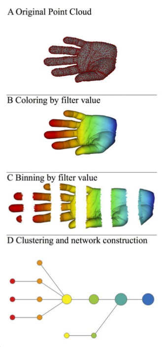
We will focus on the article [2] in the references. It allows to have an idea of the shape of the data. More precisely, we will go through the various steps that enabled the authors of [2] to produce the following figure:
Overall pipeline
The authors go through the following steps to represent the new shape:
A) A 3D object (hand) represented as a point cloud.
B) A filter value is applied to the point cloud and the object is now colored by the values of the filter function.
C) The data set is binned into overlapping groups.
D) Each bin is clustered and a network is built.
Therefore, we will need a “filter function”, a method to cluster a point cloud (the “clusterer”), N intervals and an overlap parameter. Let’s summarize this in the following class.
class TDAPipeline():

    def __init__(self, filter_function, clusterer, n, overlap):
        self._filter_function = filter_function
        self._clusterer = clusterer
        self._n = n
        self._overlap = overlap

        # (string, int list) dict
        self._clusters = []

        # string list
        self._clusters_names = []

        # (string, string) list
        self._edges = []
We are now ready to dig in the other concepts.
The filters
Filter functions allows to associate real valued quantities to the data points. It can be the coordinates of a point on any axis, or the coordinates of the points on the first component of a PCA.
class AxisFilter():

    def __init__(self, i):
        self._i = i

    def Fit(self, data):
        pass

    def Filter(self, data):
        return data[:,self._i]
An interesting discovery in this article is the concept of “L-infinity centrality”. This filter allows to associate to a point a real number qualifying how close it is to the boundary of the cloud.
L-infinity centrality, is defined for a data point x to be the maximum distance from x to any other data point in the set. Large values of this function correspond to points that are far from the center of the data set.
import numpy as np
from scipy.spatial.distance import pdist, squareform

class LinfinityCentrality():

    def __init__(self, distance):
        self._distance = distance


    def Fit(self, data):
        # Barnes Hut approx. or something similar may speed up the filtering part later
        pass


    def Filter(self, data):
        pairwise_dist = squareform(pdist(data, self._distance))
        return np.amax(pairwise_dist, axis = 1)
The clustering
Once the points have been associated to an interval in the image of the filter function, they have to be clustered. The authors use the following method:
We first construct the single linkage dendrogram for the data in the bin, and record the threshold values for each transition in the clustering. We select an integer k, and build a k-interval histogram of these transition values. The lustering is performed using the last threshold before the first gap in this histogram.
Which can be implemented taking advantage of the implementation of the single linkage proposed in scipy.
import numpy as np
from sklearn.cluster import AgglomerativeClustering
from scipy.cluster.hierarchy import fcluster, linkage

class SingleLinkageClusterer():

    def __init__(self, k):
        self._k = k

    def Cluster(self, data):
        if data.shape[0] == 0:
            return []

        linkage_matrix = linkage(data)
        counts, thresholds = np.histogram(linkage_matrix[:, 2], bins=self._k)
        first_gap_index = self._first_zero(counts, -1)
        if(first_gap_index > -0.5):
            threshold = thresholds[first_gap_index]
        else:
            threshold = linkage_matrix[-1, 2]
        clusters = fcluster(linkage_matrix, t=threshold, criterion='distance')
        return clusters

    def _first_zero(self, arr, invalid_val=-1):
        mask = arr == 0
        return np.where(mask.any(), mask.argmax(), invalid_val)
Some classical shapes
We now have what we need to follow the pipeline of the author. Let’s just sample some points from various shapes with the following classes:
class Sampler():

    def __init__(self):
        raise NotImplemented()

    def Sample(self, n):
        raise NotImplemented()
It is quite easy to sample points uniformly over a sphere (up to numerical precision issues) by sampling an distribution over R^3 which is rotation invariant (here, three independant gaussian with same mean and variance) and normalize it.
import numpy as np
from sklearn.preprocessing import normalize
from Sampler import Sampler


class SphereSampler(Sampler):

    def __init__(self, r=1):
        self._r = r

    '''
    Uniform sampling over the sphere.
    '''
    def Sample(self, n):
        mat = np.random.randn(n, 3)
        return self._r * normalize(mat, axis=1, norm='l2')
I could not find a uniform distribution over the torus, but this should be “uniform enough”.
import numpy as np
from Sampler import Sampler


class TorusSampler(Sampler):

    def __init__(self, r=1, R=3, x0=0, y0=0, z0=0):
        self._r = r
        self._R = R
        self._x0 = x0
        self._y0 = y0
        self._z0 = z0

    '''
    This sampling may not be uniform
    '''
    def Sample(self, n):
        u = 2 * np.pi * np.random.rand(n)
        v = 2 * np.pi * np.random.rand(n)

        cosu = np.cos(u)
        sinu = np.sin(u)

        cosv = np.cos(v)
        sinv = np.sin(v)

        x = self._x0 + (self._R + self._r * cosu) * cosv
        y = self._y0 + (self._R + self._r * cosu) * sinv
        z = self._z0 + self._r * sinu

        return np.array([x, y, z]).T
Experiments
Following the method of the authors
We are now ready to implement the full pipeline and produce sensible graphs.
import numpy as np


class TDAPipeline():

    def __init__(self, filter_function, clusterer, n, overlap):
        self._filter_function = filter_function
        self._clusterer = clusterer
        self._n = n
        self._overlap = overlap

        # (string, int list) dict
        self._clusters = []

        # string list
        self._clusters_names = []

        # (string, string) list
        self._edges = []

    def Run(self, data):
        self._filter_function.Fit(data)

        # one dimensional array : f(data), f : R^n -> R
        filtered_data = self._filter_function.Filter(data)
        lb = np.min(filtered_data)
        ub = np.max(filtered_data)
        overlapping_intervals = self._generate_overlapping_intervals(
            lb, ub, self._n, self._overlap)

        # f^-1([a,b]) for [a,b] in the overlapping intervals
        sliced_clusters = []
        i = 0
        for interval in overlapping_intervals:
            in_interval = map(lambda x: self._between_pair(
                x, interval), filtered_data)
            indices = np.where(in_interval)[0]
            filtered_points = data[indices, :]
            clusters = self._clusterer.Cluster(filtered_points)
            points_by_cluster = self._to_dict_list(
                str(i) + "_", indices, clusters)
            sliced_clusters.append(points_by_cluster)
            i = i + 1

        self._clusters = self._flatten_dict_list(sliced_clusters)
        self._clusters_names = self._clusters.keys()
        self._edges = self._build_edges(sliced_clusters)

        return self._edges

    def ClusterAverage(self, target):
        if len(self._clusters) == 0:
            raise "The algorithm has not been trained!"

        indices_dict = self._clusters

        return [np.mean(target[indices_dict[n]]) for n in self._clusters_names]

    def _build_edges(self, sliced_clusters):
        edges = []
        for sets_prev in sliced_clusters:
            for sets_new in sliced_clusters:
                for prev_key in sets_prev.keys():
                    for new_key in sets_new.keys():
                        if not set(sets_new[new_key]).isdisjoint(set(sets_prev[prev_key])):
                            edges.append((prev_key, new_key))
        return edges

    def _flatten_dict_list(self, dict_list):
        res = {}
        for dicts in dict_list:
            res.update(dicts)
        return res

    def _to_dict_list(self, prefix, vector, clusters):
        cluster_names = np.unique(clusters)
        res = {}
        for cluster_name in cluster_names:
            indices_in_cluster = map(lambda x: cluster_name == x, clusters)
            points_in_cluster = vector[np.where(indices_in_cluster)[0]]
            res.update({prefix + str(cluster_name): points_in_cluster})
        return res

    def _generate_overlapping_intervals(self, lb, ub, n, overlap):
        step = 1. * (ub - lb) / n
        res = [(lb + i * step - overlap * step, lb + (i + 1)
                * step + overlap * step) for i in range(n)]
        return res

    def _between_pair(self, x, pair):
        a, b = pair
        return x > a and x < b
Illustrations
Did it work :) ? I found a hand data set “Free realistic hand” here, it required a little bit of parsing to put it in a 3d file.
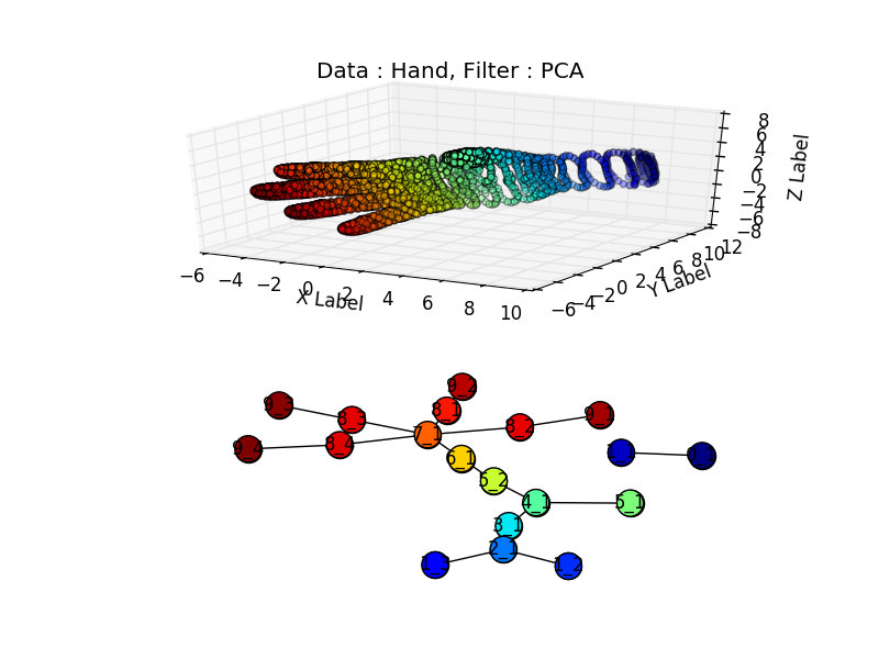
Unfortunately the sampling around the wrist is not high enough and the wrist is associated to the two blue dots, separated from the rest of the figure., but we do recognize the four fingers(in red) well separated from the thumb (in green).
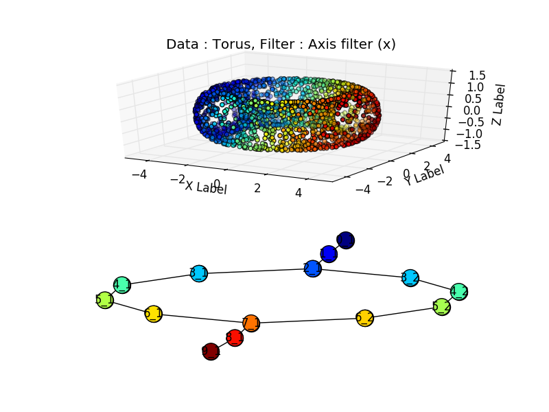
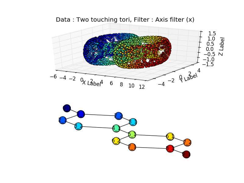
But we can generate synthetic data to get rid of this sampling issue. Per example, with a torus:
Or two touching tori:
import numpy as np

from AxisFilter import AxisFilter
from PCAFilter import PCAFilter
from LinfinityCentrality import LinfinityCentrality

from SingleLinkageClusterer import SingleLinkageClusterer

from TesseractSampler import TesseractSampler
from TorusSampler import TorusSampler
from SphereSampler import SphereSampler

from TDAPipeline import TDAPipeline

from mpl_toolkits.mplot3d import Axes3D
import matplotlib.pyplot as plt

import networkx as nx
from networkx.drawing.nx_agraph import graphviz_layout


def plot_tda_pipeline(title, sample, filter_function, clusterer, N, OVERLAP):
    tdap = TDAPipeline(filter_function, clusterer, N, OVERLAP)
    edges = tdap.Run(sample)

    colors = filter_function.Filter(sample)
    cluster_colors = tdap.ClusterAverage(colors)

    fig = plt.figure()
    ax = fig.add_subplot(211, projection='3d')

    x = sample[:, 0]
    y = sample[:, 1]
    z = sample[:, 2]

    ax.scatter(x, y, z, c=colors, marker='o')

    ax.set_xlabel('X Label')
    ax.set_ylabel('Y Label')
    ax.set_zlabel('Z Label')

    plt.title(title)
    fig.add_subplot(212)

    G = nx.OrderedGraph() # withouth OrderedGraph, the nodes may be shuffled (and the colors would not match)
    G.add_nodes_from(tdap._clusters_names)
    G.add_edges_from(edges)
    pos = graphviz_layout(G)
    nx.draw(G, pos, with_labels = True)
    nx.draw_networkx_nodes(G, pos,
            node_color = cluster_colors)

    plt.savefig(title)


N = 10
OVERLAP = 0.2
SAMPLE_SIZE = 2000
K = 5

named_samples = [("Torus", TorusSampler(1, 3).Sample(SAMPLE_SIZE)),
       ("Tesseract", TesseractSampler().Sample(SAMPLE_SIZE)),
        ("Two Spheres", np.vstack((SphereSampler().Sample(SAMPLE_SIZE),
                                            SphereSampler(3).Sample(SAMPLE_SIZE)))),
                 ("Two touching tori", np.vstack((TorusSampler(1, 3).Sample(SAMPLE_SIZE),
                                                  TorusSampler(1, 3, 6, 0, 0).Sample(SAMPLE_SIZE)))),
                 ("Hand", np.loadtxt("./Hand.csv", delimiter=","))]

named_filters = [("Axis filter (x)", AxisFilter(0)),
                 ("PCA", PCAFilter()),
                 ("L-Linfinity Centrality", LinfinityCentrality('euclidean'))]

for named_filter in named_filters:
    name_filter, filter_function = named_filter
    for named_sample in named_samples:
        name_data, sample = named_sample
        title = "Data : " + name_data + ", " + "Filter : " + name_filter
        plot_tda_pipeline(title, sample, filter_function,
                          SingleLinkageClusterer(K), N, OVERLAP)
References
Books
- Computational Topology: An Introduction by Herbert Edelsbrunner and John L. Harer
- Topological Data Analysis for Scientific Visualization (Mathematics and Visualization) by Julien Tierny
- Topology for Computing by Afra J. Zomorodian
- The elements of statistical learning by Trevor Hastie, Robert Tibshirani, Jerome Friedman
Articles
[1]F. Chazal and B. Michel, “An introduction to Topological Data Analysis: fundamental and practical aspects for data scientists,” arXiv:1710.04019 [cs, math, stat], Oct. 2017.
[2]P. Y. Lum et al., “Extracting insights from the shape of complex data using topology,” Scientific Reports, vol. 3, no. 1, Dec. 2013.
[3]B. Zieliński, M. Lipiński, M. Juda, M. Zeppelzauer, and P. Dłotko, “Persistence Bag-of-Words for Topological Data Analysis,” arXiv:1812.09245 [cs, math, stat], Dec. 2018.
[4]A. Zomorodian, “Topological Data Analysis,” p. 39.
[5]J. Mathews, S. Nadeem, M. Pouryahya, A. Tannenbaum, and J. O. Deasy, “Topological Data Analysis of PAM50 and 21-Gene Breast Cancer Assays:,” bioRxiv, Nov. 2018.