(Updated 22nd march 2021: added datasource.ai)

Here is, to my knowledge, the most complete list of data science competition platforms with sponsored (paid) competitions.

If you are not familiar with them, they are, to me, the best way to learn data science. Most of them have a dedicated community and many tutorials, starter kits for competitions. They are also a way to use your skills on topics your day job may not propose you.

If I forgot any platform, or if a link is dead, please let me know in the comments or via email, I plan to keep this article as updated as possible!

ML contests: an aggregator

ML contests

Clear. A list of competitions, by topics (NLP / supervised learning / vision …)

I am not sure all the platforms are showed here (I did not find references to numer.ai or Bitgrit, per example)

Prediction

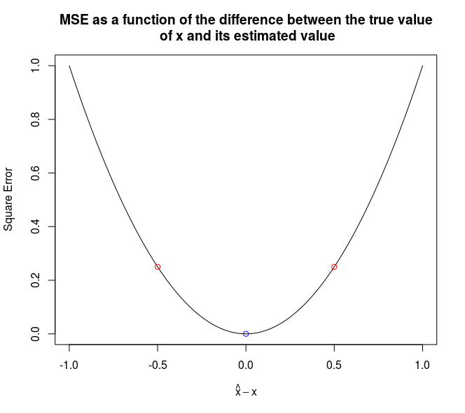
The principle here is simple, you have a train set and a test set to download (though the new trend is encouraging to push your code directly in a dedicated environment hosted by the platform).

The train set contains various columns, or images, or executables (or anything else probably) and the purpose is to predict another variable (which can be a label for classification problems, a value for regression, a set of labels for multiclass classification problem or other things, I am just focusing on the most common tasks)

Then, you upload your predictions (or your code, depending on the competition) and you get a value: the accuracy of your model on the test set. The ranking is immediate, making these platforms delightfully and dangerously addictive!

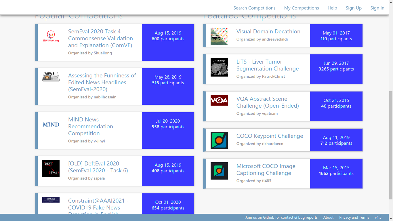
Kaggle

Kaggle competitions

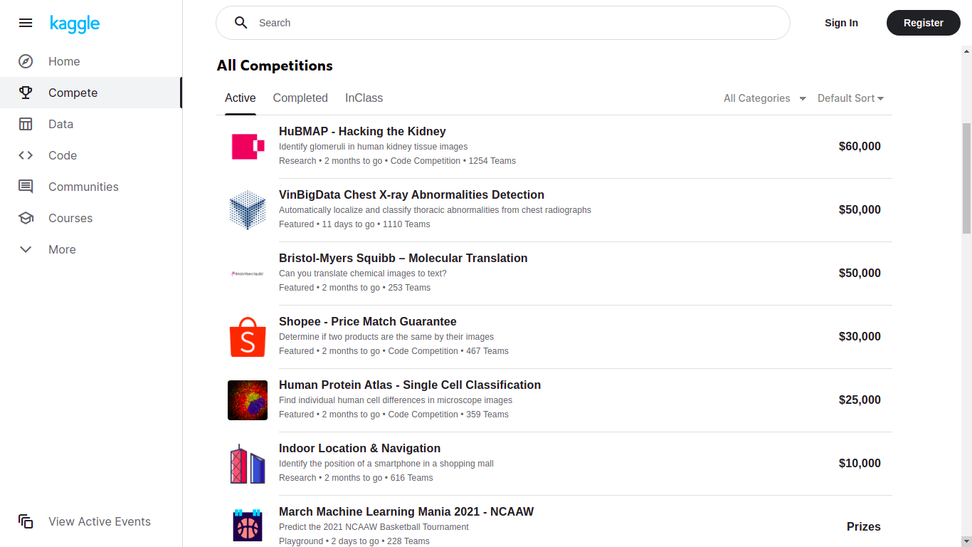
Kaggle is probably the largest platform hosting competitions, with the highest prizes and the largest community and resources. Beware, the higher the price, the harder the competition!

They also have the most complete set of learning resources and usable datasets.

AIcrowd (or CrowdAI)

AIcrowd challenge page

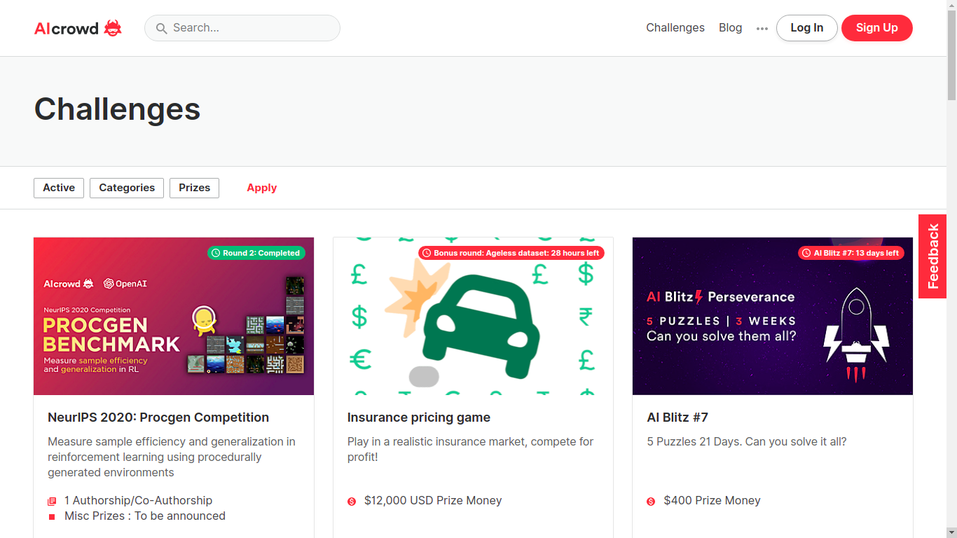
Great platform, super active, many competitions and great topics! They are growing fast so expect even more competitions to happen here.

Besides, from the competitions I have seen here, they focus on less “classical” topics than the ones you would see on Kaggle. Some may like it, others may not, I personnally do.

AIcrowd enables data science experts and enthusiasts to collaboratively solve real-world problems, through challenges.

Bitgrit

Bitgrit competitions

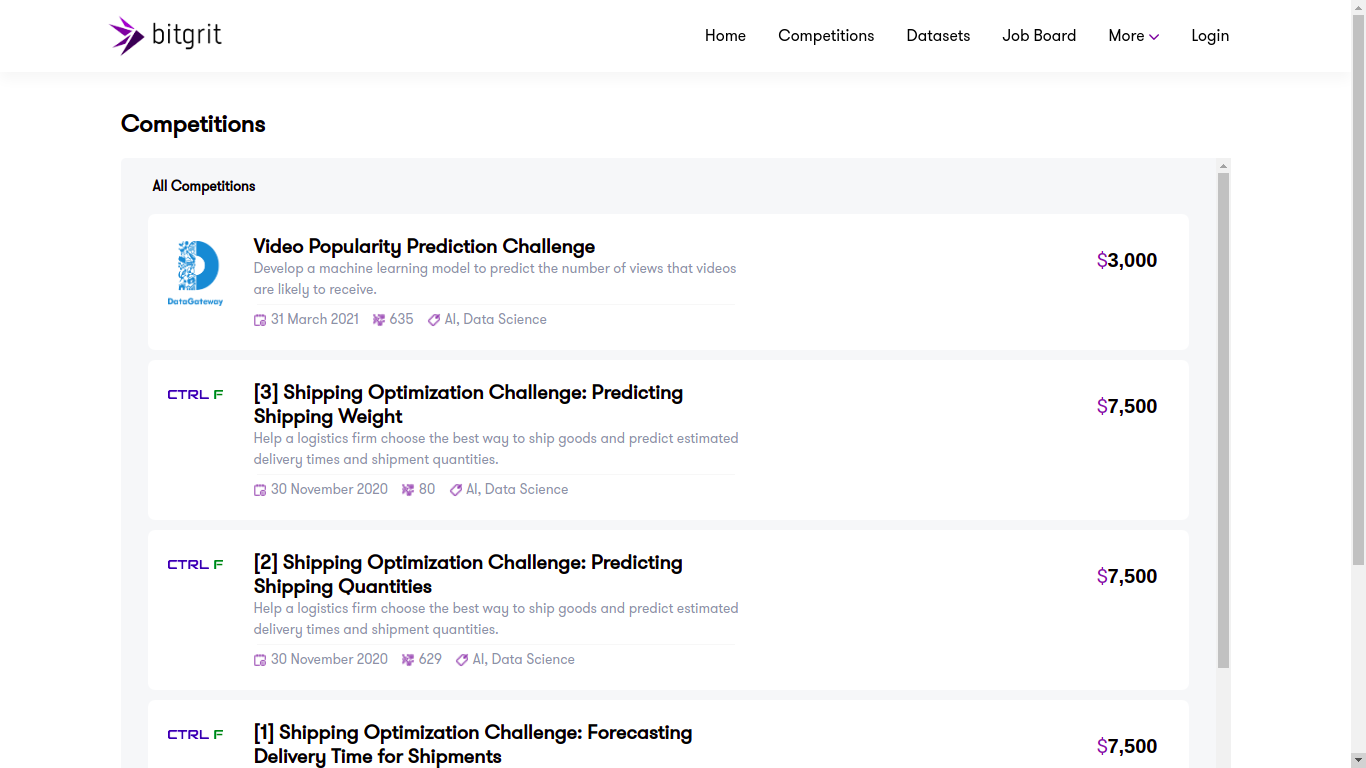
Launched in 2019, already showing 8 competitions with various topics, this platform looks promising! As said above, it does not seem referenced on mlcontests.

bitgrit is an AI competition and recruiting platform for data scientists, home to a community of over 25,000 engineers worldwide. We are developing bitgrit to be a comprehensive online ecosystem, centered around a blockchain-powered AI Marketplace.

Drivendata

Driven data competition page

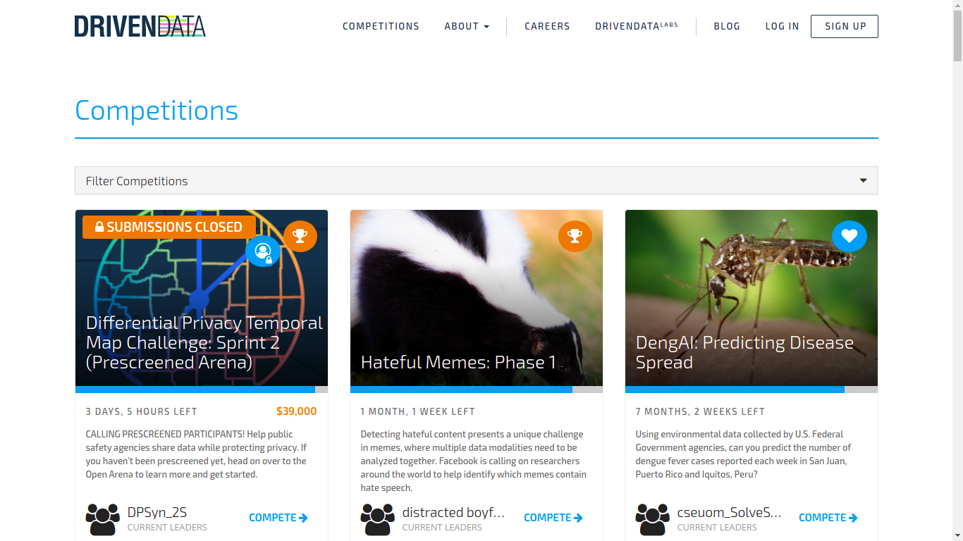
I never took part in their competitions, so I can’t say mcuh about it for now! But they have sponsored competitions.

DrivenData works on projects at the intersection of data science and social impact, in areas like international development, health, education, research and conservation, and public services. We want to give more organizations access to the capabilities of data science, and engage more data scientists with social challenges where their skills can make a difference.

Crowdanalytix

Crowdanalytix

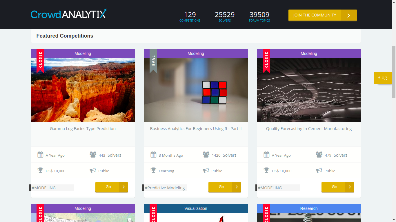
I never took part in their competitions, so I can’t say mcuh about it for now! They seemed less active recently, but they had sponsored competitions.

25,129 + Data Scientists

102,083 + Models Built

50 + Countries

Numer.ai

https://numer.ai/

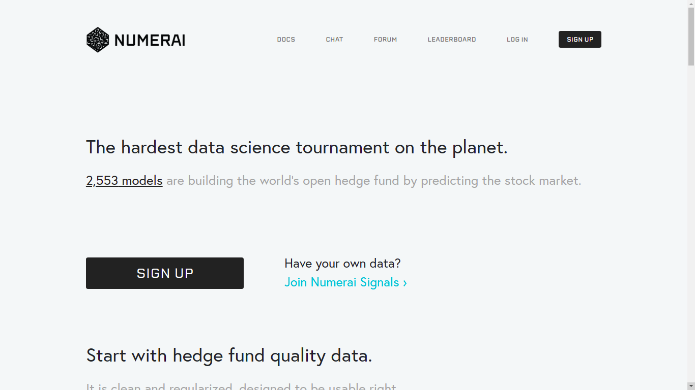
Focusing on predicting the stock market, with high quality data (which is usually a tedious task when you try to have quality data in finance). They claim to be the hardest platform in finance, and having worked there, I can confirm that finding the slightest valuable prediction is super hard!

Nice if you like finance, but be prepared to work with similar datasets!

Start with hedge fund quality data. It is clean and regularized, designed to be usable right away.

Zindi

Zindi competition page

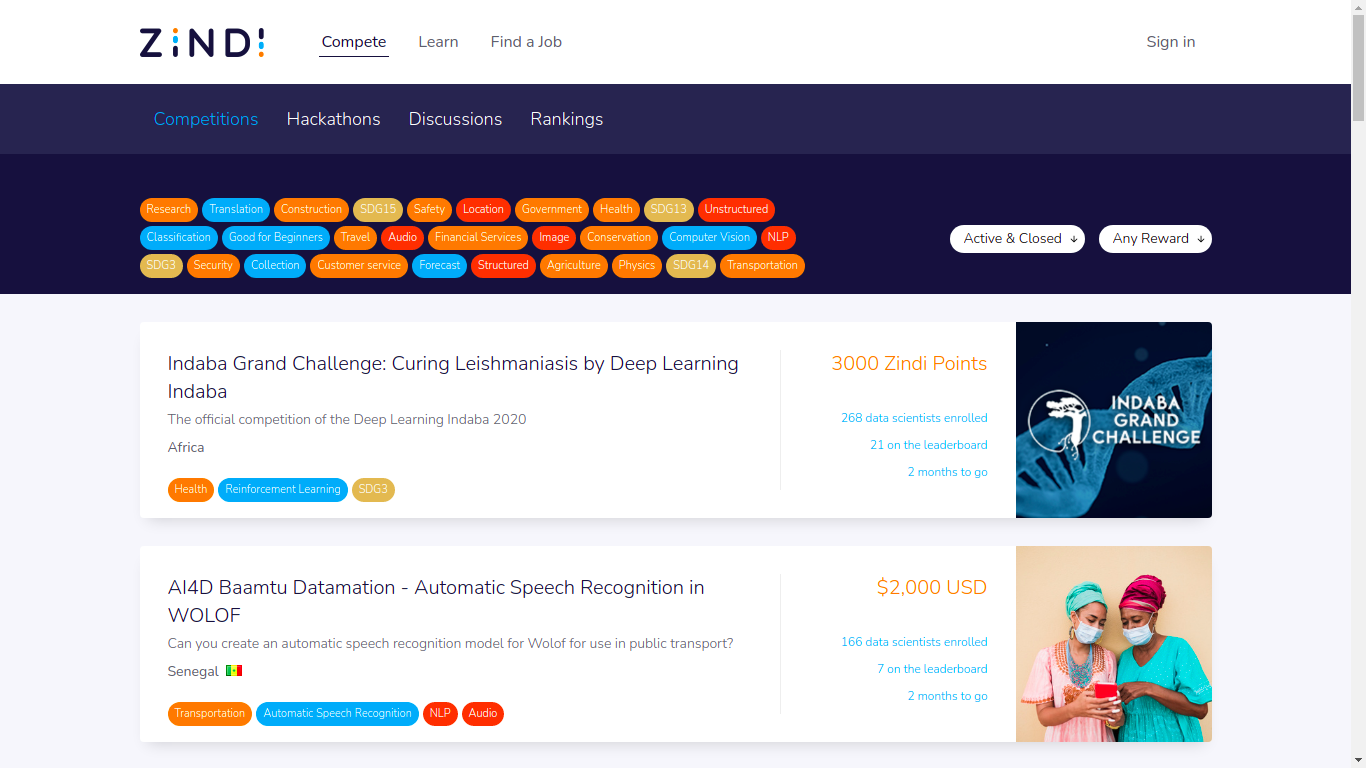
Data science platform with competitions which are related to Africa. The NLP part seems particularly exciting, as they are focus on languages which are not studied as often as English or Spanish! Looking forward to participate in one of their challenges!

We connect organisations with our thriving African data science community to solve the world’s most pressing challenges using machine learning and AI.

Analytics Vidhya

Analytics Vidhya

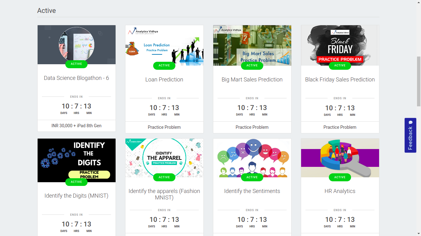
India based.

Data science hackathons on DataHack enable you to compete with leading data scientists and machine learning experts in the world. This is your chance to work on real life data science problems, improve your skill set, learn from expert data science and machine learning professionals, and hack your way to the top of the hackathon leaderboard! You also stand a chance to win prizes and get a job at your dream data science company.

Challengedata

https://challengedata.ens.fr/

Not sure the competitions are sponsored here. General topics, most of them seem to come from French companies and French institutions.

We organize challenges of data sciences from data provided by public services, companies and laboratories: general documentation and FAQ. The prize ceremony is in February at the College de France.

Coda Lab

Codalab

French based.

CodaLab is an open-source platform that provides an ecosystem for conducting computational research in a more efficient, reproducible, and collaborative manner.

Topcoder

Topcoder

Not focusing only on data science:

Access our community of world class developers, great designers, data science geniuses and QA experts for the best results

InnoCentive

InnoCentive competitions

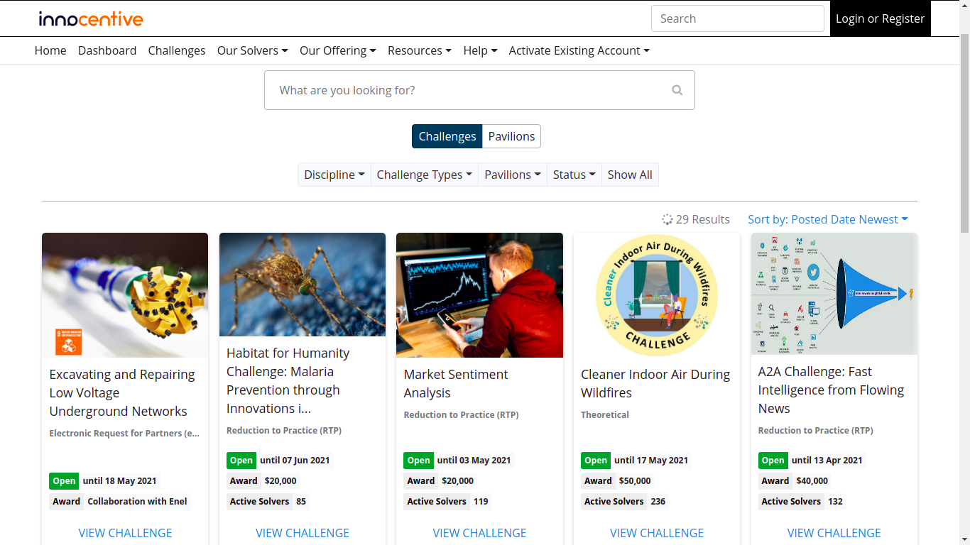
InnoCentive is the global pioneer in crowdsourced innovation. We help innovative organizations solve their important technology, science, business, A/I and data challenges by connecting them with a global network of expert problem solvers.

Datasoure.ai

Datasoure

Young company, as the quote below shows (22nd march 2021). They seem to be focused on challenges for startups, but this may evolve!

At a glance

2 Team Members

1,692 Data Scientists

12 Companies

5.2% Weekly Growth

Signate

Signate competitions

A Japanese competition platform. Most of the competitions are described in Japanese, but not all of them!

SIGNATE collaborates with companies, government agencies and research institutes in various industries to work on various projects to resolve social issues. We invite you to join SIGNATE’s project, which aims to make the world a better place through the power of open innovation.

datasciencechallenge.org (probably down)

https://www.datasciencechallenge.org/

Unfortunately, I cannot reach the website any more…

Sponsored by the Defence Science and Technology Laboratory and other UK government departments.

datascience.net (probably down for ever)

datascience.net

Used to be a French speaking data science competition for a while. However, the site has been down for a while now… Worth giving a look from time to time!

Dataviz

Here, the idea is to provide the best vizualisation of datasets. The metric may therefore not be as absolute as the one for prediction problems and the skillset is really different!

Iron viz

Iron viz

informationisbeautifulawards

informationisbeautifulawards

They are all the platforms I am aware of, if I missed any or if you have any relevant resources, please let me know!

I Hope you liked this article! If you plan to take part in any of these competitions, best of luck to you, and have fun competing and learning!

As I was renewing my domain name, I figured out I had been posting here for quite a while now :) at a completely irregular frequency, I must admit. Anyways, thank you to all of the readers for your support and interest in my articles ! It was really pleasant to read the various comments or mails you sent me.

As for the blog itself, well, I learnt a lot. About machine learning, obviously, but also about this thing called SEO. I am a little bit surprised by the success of some articles and the oblivion others fell into, but I guess this is how referencing works. One of my most read articles is python plot 3d scatter and density though it did not take much time to write, while a stacking tutorial in Python and theory behind model stacking seem to be invisible from a search engine point of view… But I am not here to rant.

The plan, if any, is to keep posting articles about all the aspects of machine learning which I consider interesting ! I have some material for the decision boundaries of common machine learning algorithms, some code for decision trees, random forest and parallel computations in OCaml and more data visualization snippets…

Another thing, if you like my content and want to support me, I joined the Brave creators program. So if you use this browser and want to help, I would gladly receive BAT tips! Thanks to the anonymous donors who already contributed.

And as usual, if you have some topics you are curious about, some tutorials you would like to read, just let me know in the comments or by mail, I will see what I can do!

Have a nice day!

Model staging is a method that enables to produce (usually) the most competitive models, in terms of accuracy. As such, you will often find winning solutions to data science competitions to be 2-3 stages of models.

This article will assume some familiarity with cross validation. We will go through model averaging first, recall how staging works, observe the link between model averaging and model staging (also referred to as stacking or blending) and propose hypothesis (backed by some visualization) to explain why staging works so well.

Also my other post (more implementation oriented), a stacking tutorial in Python may help.

Going back to model staging, here are some verbatim about some winning solutions of data science competitions.

Per example, the Homesite quote conversion

Quick overview for now about the NMA approach:

10 variations of the dataset in total (factor combinations, factors mapped to response rates, replacing correlated pairs by differences etc) lots of models (xgboost, keras, ranger, logreg, even occasional svm - although that took forever) trained on various datasets and different params; stored as lvl1 metafeatures mix lvl1 metafeatures with: xgboost, nnet, hillclimbing, glmnet and ranger, stack - 5 lvl2 metafeatures mix the lvl2 metafeatures with hillclimbing bag at each stage as much as time permitted

Or, in the BNP Paribas Cardif Claims management:

We also produced many different base level models without much Feature engineering, just different input format types (like load all categorical variables as counts, or as onehot encoding etc).

Our ensemble was consisted of 223 models. Faron did a lot of work in removing noise and discarding many of these in order to get to our bets score with a lvl2 ensemble of geomean weights between an ET , 2NN and 2 Xgmodels.

Before understanding the mechanisms at work for model staging, let’s review the simpler “model averaging” approach.

Model averaging

What is model averaging?

Model averaging is a method that consists in averaging the predictions of different models.

It works particularly well in regression problems, or classification problem when the task consists in predicting probabilities of belonging to a specific class.

Why does averaging works?

Imagine you are facing a regression problem, and have two models. One underestimates the true value, while the other one overestimates it. In this case, the average of the two predictions will be (much) closer to the truth than each individual prediction.

The two figures below illustrate it, in the case of a squared error penalty. The x-axis represents the difference between the true value and the estimated value. The red dots are the estimations of two different models (on the x axis) and the resulting error (on the y axis). The component of the blue dot on the x-axis is the average of the components of the red dots on the x-axis.

It is worth noting that blending will work better if the models have a similar performance (in terms of out-of-sample accuracy) and are as little correlated as possible.

Jensen inequality

What is even better is that if both models overestimate (or underestimate) the true value, the penalty is still lower.

The graph below presents it:

The green point correpond to the average of the errors, while the blue point correspond of the error of the average.

Proofs can be found on Wikipedia for the purpose of the article, it is enough to convice oneself that this works with these simple graphs.

Jensen’s inequality applies to convex functions, but log loss, squared error (MSE), absolute value error (MAE) are convex functions.

The R code below can be used (just change the xs_points <- c(0.1, 0.8)) to reproduce the experiment with other values.

parabola = function(x) {
  x * x
}
xs <- seq(-1, 1, 0.01)
xs_points <- c(0.1, 0.8)

plot(
  xs,
  parabola(xs),
  xlab = expression(hat(x) - x),
  ylab = "Square Error",
  type = 'l',
  main = "MSE as a function of the difference between the true value\n of x and its estimated value"
)

for (xs_point in xs_points) {
  points(x = xs_point,
         y = parabola(xs_point),
         col = "red")
}

points(x = mean(xs_points),
       y = parabola(mean(xs_points)),
       col = "blue")
segments(
  x0 = xs_points[1],
  x1 = xs_points[2],
  y0 = parabola(xs_points[1]),
  y1 = parabola(xs_points[2]), lty = 11
)
points(x = mean(xs_points),
       y = mean(parabola(xs_points)),
       col = "green")

Model stacking

Historical note

As far as I know, the first presentation of stacking goes back to 1992: Stacked generalization, by David H. Wolpert (also famous for the result no free lunch in search and optimization)

[…] The conclusion is that for almost any real-world generalization problem one should use some version of stacked generalization to minimize the generalization error rate.

And almost 30 years later, it remains true! Quoting the wikipedia page:

This work was developed further by Breiman, Smyth, Clarke and many others, and in particular the top two winners of 2009 Netflix competition made extensive use of stacked generalization (rebranded as “blending”)

How does it work?

Generalizing averaging

So far, we have seen model averaging. You take two models (or \(n\)), and average them.

On the other hand, assuming you cross validate \(n\) models and only use the best for future predictions, you have another strategy that forms one model from \(n\) models.

So we have two schemes that put weights on different models. One puts an equal weight to every model, the other one puts all the weights on the best model.

Model staging consists in using another learning algorithm to choose the “weights” to give to each model. A linear regression “on top” of other models consists in giving an “ideal” (in the regression sense) weight to each model, but what is amazing is that you may use something else than a linear regression!

Detailing staging procedure

The idea, to give a correct “weight” to each model is to perform a cross validation on the training set and return a dataset for which each element correspond to the unseen fold prediction. On this new dataset, you can fit the new model.

Per example, in the case of a regression problem, if you have \(n\) rows in your data set, \(p\) features and \(k\) models, this step turns your training data from a \(n,p\) matrix to a \(n,k\) matrix.

Thus the element with index \(i,j\) in this new matrix corresponds to the prediction of the \(i\)-th observation by the \(j\)-th model.

Why does this work?

General case of averaging

Averaging, because of Jensen’s inequality, usually improves the accuracy of the models. Staging, seen as a generalization of averaging, will also improve the accuracy of our learners.

More general decision boundaries

Hypothesis

Another argument, which could be rephrased in more scientific terms is that it allows to obtain decision boundaries of a wider shape than the ones of each usual learning algorithm.

Put another way, the supervised learning problems can be seen as finding \(f\) such that:

Where \(f\) belongs to some function space. For the linear regressions (penalized or not), \(f\) has to be a linear function, for a decision tree, \(f\) belongs to a space of sum of indicator functions, for kernel functions, \(f\) is a linear combination of kernels…

The hypothesis here is that, in the case of averaging, \(f\) can be linear in some region, constant by pieces in another, etc, making the search space for \(f\) larger than the search space of all the single families of models.

Visualization

As expected, the decision tree has a decision boundary consisting of segments parallel to the x and y axis.

The SVC on the other hand has a very smooth decision boundary.

And here comes the magic, the decision boundary is “a little bit of both”.

Same when we blend with a decision tree.

Code

I use the default stacking proposed by scikit-learn.

First a small class useful to plot decision boundaries.

import numpy as np
import matplotlib.pyplot as plt


class DecisionBoundaryPlotter:

    def __init__(self, X, Y, xs=np.linspace(0, 1, 30),
                 ys=np.linspace(0, 1, 30)):
        self._X = X
        self._Y = Y
        self._xs = xs
        self._ys = ys

    def _predictor(self, model):
        model.fit(self._X, self._Y)
        return (lambda x: model.predict_proba(x.reshape(1,-1))[0, 0])

    def _evaluate_height(self, f):
        fun_map = np.empty((self._xs.size, self._ys.size))
        for i in range(self._xs.size):
            for j in range(self._ys.size):
                v = f(
                    np.array([self._xs[i], self._ys[j]]))
                fun_map[i, j] = v
        return fun_map

    def plot_heatmap(self, model, name):
        f = self._predictor(model)
        fun_map = self._evaluate_height(f)

        fig = plt.figure()
        s = fig.add_subplot(1, 1, 1, xlabel='$x$', ylabel='$y$')
        im = s.imshow(
            fun_map,
            extent=(self._ys[0], self._ys[-1], self._xs[0], self._xs[-1]),
            origin='lower')
        fig.colorbar(im)
        fig.savefig(name + '_Heatmap.png')
    
    def plot_contour(self, model, name):
        f = self._predictor(model)
        fun_map = self._evaluate_height(f)

        fig = plt.figure()
        s = fig.add_subplot(1, 1, 1, xlabel='$x$', ylabel='$y$')
        s.contour(self._xs, self._ys, fun_map, levels = [0.5])
        s.scatter(self._X[:,0], self._X[:,1], c = self._Y)
        fig.suptitle(name)
        fig.savefig(name + '_Contour.png')

The plots (yeah, the nested named models is not that elegant):

import numpy as np
from sklearn.ensemble import RandomForestClassifier, ExtraTreesClassifier, AdaBoostClassifier
from sklearn.tree import DecisionTreeClassifier
from sklearn.svm import SVR, SVC
from sklearn.neighbors import KNeighborsClassifier  
from sklearn.linear_model import LogisticRegression
from sklearn.ensemble import StackingClassifier
from DecisionBoundaryPlotter import DecisionBoundaryPlotter


def random_data_classification(n, p, f):
    predictors = np.random.rand(n, p)
    return predictors, np.apply_along_axis(f, 1, predictors)


def parabolic(x, y):
    return (x**2 + y**3 > 0.5) * 1


def parabolic_mat(x):
    return parabolic(x[0], x[1])


X, Y = random_data_classification(300, 2, parabolic_mat)

dbp = DecisionBoundaryPlotter(X, Y)

named_classifiers = [ (DecisionTreeClassifier(max_depth=4), "DecisionTreeClassifier"),
                     (StackingClassifier(estimators=[
                            ("svc", SVC(probability=True)), 
                            ("dt", DecisionTreeClassifier(max_depth=4))], 
                         final_estimator=LogisticRegression()), 
                         "Stacked (Linear)"),
                     (StackingClassifier(estimators=[
                            ("svc", SVC(probability=True)), 
                            ("dt", DecisionTreeClassifier(max_depth=4))], 
                         final_estimator=DecisionTreeClassifier(max_depth=4)), 
                         "Stacked (Decision Tree)"),
                     (SVC(probability=True), "SVC")]

for named_classifier in named_classifiers:
    print(named_classifier[1])
    dbp.plot_contour(named_classifier[0], named_classifier[1])

Learning more and references

The elements of statistical learning by Trevor Hastie, Robert Tibshirani, Jerome Friedman is a brilliant introduction to machine learning and will help you have a better understanding of cross validation and the learning algorithms presented here (SVC, Decision trees) but unfortunately does not treat model staging.

You may need to extract trees from a classifier for various reasons. In my case, I thought that the feature of xgboost ntree_limit was quite convenient when cross validating a gradient boosting method over the number of trees.

What it does is that it only uses the first ntree_limit trees to perform the prediction (instead of using all the fitted tree).

predict(data, output_margin=False, ntree_limit=0, pred_leaf=False, 
        pred_contribs=False, approx_contribs=False, 
        pred_interactions=False, validate_features=True, training=False)

And it is also available as an extra argument of .predict() if you use the scikit-learn interface :

ypred = bst.predict(dtest, ntree_limit=bst.best_ntree_limit)

Indeed, by doing so, if you want to find the optimal number of trees for your model, you do not have to fit the model for 50 trees, and then predict, then fit it for 100 trees and then predict. You may fit the model once and for all for 200 trees and then, playing with ntree_limit you can observe the performance of the model for various number of trees.

The RandomForest, as implemented in scikit-learn does not show this parameter in its .predict() method. However, this is something we can quickly fix. Indeed, the RandomForest exposes estimators_. You can modify it (beware, this is a bit hacky and may not work for other versions of scikit-learn).

rf_model = RandomForestRegressor()
rf_model.fit(x, y)

estimators = rf_model.estimators_

def predict(w, i):
    rf_model.estimators_ = estimators[0:i+1]
    return rf_model.predict(x)

And that’s it, the predict method now only looks at the first i trees ;)

What is stacking and why using it

Introduction

In the case of supervised learning, stacking is a process that enables to improve the performance of a predictor. It can be used for classification and regression problems. If you took part in statistics competitions, you may already be familiar with it, but the resources about this technique are quite scarce on the internet.

From blending to stacking

As with blending, where a simple average between models with similar performance often proposes a model whose performance is higher than the one of each model in the blend, stacking combine models in a way that is dependant on the training set.

Stacking can be thought as “the sequel” of blending. Imagine you have two models with a similar performance on a dataset. The simplest blend consists in averaging the two models. However, you may become curious and propose different weight for each model. Per example, a blending with a weight of 0.7 for the first model predictions and 0.3 for the second may be better than the default 50/50 weights.

Now let’s suppose you have \(n\) models and are looking for the best weights for these n models. The problem you are facing now becomes to performing a linear regression, doesn’t it ?

The only difference is that you cannot use the prediction on the training set directly (where some models like Random Forests usually have a perfect accuracy). This is where stacking comes in!

When do you need stacking ?

Staging is usually the winning solution of many data science competitions.

Per example, the Homesite quote conversion

Quick overview for now about the NMA approach:

10 variations of the dataset in total (factor combinations, factors mapped to response rates, replacing correlated pairs by differences etc) lots of models (xgboost, keras, ranger, logreg, even occasional svm - although that took forever) trained on various datasets and different params; stored as lvl1 metafeatures mix lvl1 metafeatures with: xgboost, nnet, hillclimbing, glmnet and ranger, stack - 5 lvl2 metafeatures mix the lvl2 metafeatures with hillclimbing bag at each stage as much as time permitted

I will come back to the notions of lv1 / lvl2… stages

Or, in the BNP Paribas Cardif Claims management:

We also produced many different base level models without much Feature engineering, just different input format types (like load all categorical variables as counts, or as onehot encoding etc).

Our ensemble was consisted of 223 models. Faron did a lot of work in removing noise and discarding many of these in order to get to our bets score with a lvl2 ensemble of geomean weights between an ET , 2NN and 2 Xgmodels.

And there are plenty of other examples. So basically, stacking comes in when the accuracy of your classifier or regressor is the essence of your problem. It makes the interpretability of the model really low and is harder to implement and deploy than a simple machine learning pipe.

Principles of stacking

The idea, to give a correct weight to each model is to perform a cross validation on the training set and return a dataset for which each element correspond to the unseen fold prediction. On this new dataset, you can fit the new model.

Per example, in the case of a regression problem, if you have \(n\) rows in your data set, \(p\) features and \(k\) models, this step turns your training data from a \(n,p\) matrix to a \(n,k\) matrix.

In the case of a muli class problem, if you have \(n\) rows in your data set, \(p\) features, \(m\) classes and \(k\) models, this step turns your training data from a \(n,p\) matrix to a \(n,k \dot m\) matrix.

An example

The dataset

I will use the MNIST dataset, under a CSV format, which can be found here: on Kaggle and a logloss penalty. Of course, you will be able to play with other metrics / datasets using the code below!

The stacking / CV class

The class below can be used for a multi-class learning problem. Some minor adaptations may be required, per example for regression problems.

from sklearn.model_selection import KFold
import datetime
import pandas as pd
import numpy as np
from time import time

class bcolors:
    HEADER = '\033[95m'
    OKBLUE = '\033[94m'
    OKGREEN = '\033[92m'
    WARNING = '\033[93m'
    FAIL = '\033[91m'
    ENDC = '\033[0m'
    BOLD = '\033[1m'
    UNDERLINE = '\033[4m'


class ModelStager:

    def __init__(self, penalty, n_folds,
                 verbose=1, shuffle=True, random_state=1):
        self._penalty = penalty
        self._n_folds = n_folds
        self._verbose = verbose
        self._random_state = random_state
        self._shuffle = shuffle

    def _print(self, input_str):
        time = datetime.datetime.now().strftime("%Y-%m-%d %H:%M")
        print(bcolors.HEADER + "[ModelStager | " + time + "] " + bcolors.ENDC + str(input_str)) 

    def fit(self, X, y, model):
        kfold = KFold(n_splits=self._n_folds, shuffle=self._shuffle,
                  random_state=self._random_state)

        cv_scores = []
        oof_predictions = pd.DataFrame(index=X.index, columns=range(y.nunique()))

        fold_idx = 0

        for tr_idx, val_idx in kfold.split(X):

            X_tr = X.iloc[tr_idx]
            X_val = X.iloc[val_idx]

            y_tr = y.iloc[tr_idx]
            y_val = y.iloc[val_idx]

            if self._verbose:
                self._print("Data_tr shape : " + str(X_tr.shape))

            fold_idx = fold_idx + 1
            t = time()

            model.fit(X_tr, y_tr)

            validation_prediction = model.predict_proba(X_val)

            oof_predictions.iloc[val_idx] = validation_prediction

            cv_score_model = self._penalty(y_val, validation_prediction)
            cv_scores.append(cv_score_model)

            if self._verbose:
                self._print("Fold %.0f : TEST %.5f | TIME %.2fm (1-fold)" %
                            (fold_idx, cv_score_model, (time() - t) / 60))

        self._print("TEST AVERAGE : %.5f" % (np.mean(cv_scores)))

        return oof_predictions

As you can see, the ModelStager also performs cross validation. All the magic happens in oof_predictions, which is in charge of keeping track of the out-of-fold prediction and returning it. As mentioned earlier, it shares the index with X, and the columns correspond to the number of classes.

All the bcolors and custom printing function are just things I am used to work with, no need to bother about it.

Example

Random Forest and Extra trees

If you append this at the bottom of the previous class, you may re run the operations.

Two models are proposed, and their ensemble below (using a logistic regression).

if __name__ == "__main__":
    
    from sklearn.metrics import log_loss
    from sklearn.linear_model import LogisticRegression
    from sklearn.ensemble import RandomForestClassifier, ExtraTreesClassifier
    from xgboost import XGBClassifier

    train_data = pd.read_csv("./mnist_train.csv", nrows=5000)
    X = train_data.drop(["label"], axis=1)
    y = train_data["label"]
    
    stager = ModelStager(log_loss, 5)

    print("RF model")
    model_rf = RandomForestClassifier()
    stage1_rf = stager.fit(X, y, model_rf)

    print("ET model")
    model_et = ExtraTreesClassifier()
    stage1_et = stager.fit(X, y, model_et)

    print("Stage 1 : (RF, ET) -> logistic model")
    stage1_rf_et = pd.concat([stage1_rf, stage1_et], axis=1)
    stager.fit(stage1_rf_et, y, LogisticRegression())

Results

RF model
[ModelStager | 2021-01-07 13:54] Data_tr shape : (4000, 784)
[ModelStager | 2021-01-07 13:54] Fold 1 : TEST 0.48133 | TIME 0.05m (1-fold)
[ModelStager | 2021-01-07 13:54] Data_tr shape : (4000, 784)
[ModelStager | 2021-01-07 13:55] Fold 2 : TEST 0.44262 | TIME 0.05m (1-fold)
[ModelStager | 2021-01-07 13:55] Data_tr shape : (4000, 784)
[ModelStager | 2021-01-07 13:55] Fold 3 : TEST 0.46714 | TIME 0.05m (1-fold)
[ModelStager | 2021-01-07 13:55] Data_tr shape : (4000, 784)
[ModelStager | 2021-01-07 13:55] Fold 4 : TEST 0.45846 | TIME 0.05m (1-fold)
[ModelStager | 2021-01-07 13:55] Data_tr shape : (4000, 784)
[ModelStager | 2021-01-07 13:55] Fold 5 : TEST 0.45377 | TIME 0.05m (1-fold)
[ModelStager | 2021-01-07 13:55] TEST AVERAGE : 0.46066
ET model
[ModelStager | 2021-01-07 13:55] Data_tr shape : (4000, 784)
[ModelStager | 2021-01-07 13:55] Fold 1 : TEST 0.44834 | TIME 0.04m (1-fold)
[ModelStager | 2021-01-07 13:55] Data_tr shape : (4000, 784)
[ModelStager | 2021-01-07 13:55] Fold 2 : TEST 0.44679 | TIME 0.04m (1-fold)
[ModelStager | 2021-01-07 13:55] Data_tr shape : (4000, 784)
[ModelStager | 2021-01-07 13:55] Fold 3 : TEST 0.43367 | TIME 0.04m (1-fold)
[ModelStager | 2021-01-07 13:55] Data_tr shape : (4000, 784)
[ModelStager | 2021-01-07 13:55] Fold 4 : TEST 0.43551 | TIME 0.04m (1-fold)
[ModelStager | 2021-01-07 13:55] Data_tr shape : (4000, 784)
[ModelStager | 2021-01-07 13:55] Fold 5 : TEST 0.42378 | TIME 0.04m (1-fold)
[ModelStager | 2021-01-07 13:55] TEST AVERAGE : 0.43762
Stage 1 : (RF, ET) -> logistic model
[ModelStager | 2021-01-07 13:55] Data_tr shape : (4000, 20)
[ModelStager | 2021-01-07 13:55] Fold 1 : TEST 0.20850 | TIME 0.01m (1-fold)
[ModelStager | 2021-01-07 13:55] Data_tr shape : (4000, 20)
[ModelStager | 2021-01-07 13:55] Fold 2 : TEST 0.16870 | TIME 0.00m (1-fold)
[ModelStager | 2021-01-07 13:55] Data_tr shape : (4000, 20)
[ModelStager | 2021-01-07 13:55] Fold 3 : TEST 0.21278 | TIME 0.00m (1-fold)
[ModelStager | 2021-01-07 13:55] Data_tr shape : (4000, 20)
[ModelStager | 2021-01-07 13:55] Fold 4 : TEST 0.20536 | TIME 0.00m (1-fold)
[ModelStager | 2021-01-07 13:55] Data_tr shape : (4000, 20)
[ModelStager | 2021-01-07 13:55] Fold 5 : TEST 0.18016 | TIME 0.00m (1-fold)
[ModelStager | 2021-01-07 13:55] TEST AVERAGE : 0.19510

This is quite a huge boost ;) to be honest, this part is a little bit of an artifact, as ensemble of decision trees are usually quite bad at predicting probabilities, the logloss is artificially high. And the logistic regression corrects this phenomenon.

Random Forest, Extra Trees and Gradient Boosting

As stated above, the main performance gain comes from using an algorithm that is better at optimizing logloss.

Gradient boosting methods (most notably, xgboost) are good at predicting probability. This is illustrated when we perform the cross validation of a gradient boosting model over the original dataset.

print("XGB model")
model_xgb = XGBClassifier(use_label_encoder=False)
stage_1_xgb = stager.fit(X, y, model_xgb)

Yields the following results

XGB model
[ModelStager | 2021-01-07 13:55] Data_tr shape : (4000, 784)
[ModelStager | 2021-01-07 13:56] Fold 1 : TEST 0.21077 | TIME 1.05m (1-fold)
[ModelStager | 2021-01-07 13:56] Data_tr shape : (4000, 784)
[ModelStager | 2021-01-07 13:57] Fold 2 : TEST 0.16564 | TIME 1.15m (1-fold)
[ModelStager | 2021-01-07 13:57] Data_tr shape : (4000, 784)
[ModelStager | 2021-01-07 13:58] Fold 3 : TEST 0.25023 | TIME 1.09m (1-fold)
[ModelStager | 2021-01-07 13:58] Data_tr shape : (4000, 784)
[ModelStager | 2021-01-07 13:59] Fold 4 : TEST 0.24772 | TIME 1.03m (1-fold)
[ModelStager | 2021-01-07 13:59] Data_tr shape : (4000, 784)
[ModelStager | 2021-01-07 14:00] Fold 5 : TEST 0.18703 | TIME 1.12m (1-fold)
[ModelStager | 2021-01-07 14:00] TEST AVERAGE : 0.21228

Though much better than the single RandomForestClassifier or ExtraTreesClassifier alone, it does not beat the staged model.

Now let’s add the xgb features to the stage 1:

print("Stage 1 : (FR, ET, XGB) -> logistic model")
stage1_rf_et_xgb = pd.concat([stage1_rf, stage1_et, stage_1_xgb], axis=1)
stager.fit(stage1_rf_et_xgb, y, LogisticRegression())

And once again, the performance increases.

Stage 1 : (FR, ET, XGB) -> logistic model
[ModelStager | 2021-01-07 14:00] Data_tr shape : (4000, 30)
[ModelStager | 2021-01-07 14:00] Fold 1 : TEST 0.19343 | TIME 0.01m (1-fold)
[ModelStager | 2021-01-07 14:00] Data_tr shape : (4000, 30)
[ModelStager | 2021-01-07 14:00] Fold 2 : TEST 0.15602 | TIME 0.01m (1-fold)
[ModelStager | 2021-01-07 14:00] Data_tr shape : (4000, 30)
[ModelStager | 2021-01-07 14:00] Fold 3 : TEST 0.20996 | TIME 0.01m (1-fold)
[ModelStager | 2021-01-07 14:00] Data_tr shape : (4000, 30)
[ModelStager | 2021-01-07 14:00] Fold 4 : TEST 0.20830 | TIME 0.01m (1-fold)
[ModelStager | 2021-01-07 14:00] Data_tr shape : (4000, 30)
[ModelStager | 2021-01-07 14:00] Fold 5 : TEST 0.17053 | TIME 0.01m (1-fold)
[ModelStager | 2021-01-07 14:00] TEST AVERAGE : 0.18765

And if we include the gradient boosting predictions in the stage 1 features, the logloss drops from 0.19510 to 0.18765

More stage 1 features

I only presented 3 models in the stage 1. I could have added plenty of others, such as nearest neighbors, linear models… However, I strongly recommend to play with the code below and try to add these models, I am pretty sure than much better scores can be obtained ;)

Or I could also have performed some feature engineering for some models and not for others. As you can see, the number of combination becomes really huge. The “secret” to have a good performance after stacking is to have models that are as different (surprisingly, the performance of each model is not that important) as possible.

Beyond the linear model

I mostly referred to the stage 1 as a weighting operation, but it does not have to be a linear model. You can also use other model on top of your stage one features! Per example, another gradient boosting model, or a neural network. You can even repeat the above to produce stage 2 features, and train another model on this stage 2.

The code

from sklearn.model_selection import KFold
import datetime
import pandas as pd
import numpy as np
from time import time

class bcolors:
    HEADER = '\033[95m'
    OKBLUE = '\033[94m'
    OKGREEN = '\033[92m'
    WARNING = '\033[93m'
    FAIL = '\033[91m'
    ENDC = '\033[0m'
    BOLD = '\033[1m'
    UNDERLINE = '\033[4m'


class ModelStager:

    def __init__(self, penalty, n_folds,
                 verbose=1, shuffle=True, random_state=1):
        self._penalty = penalty
        self._n_folds = n_folds
        self._verbose = verbose
        self._random_state = random_state
        self._shuffle = shuffle

    def _print(self, input_str):
        time = datetime.datetime.now().strftime("%Y-%m-%d %H:%M")
        print(bcolors.HEADER + "[ModelStager | " + time + "] " + bcolors.ENDC + str(input_str)) 

    def fit(self, X, y, model):
        kfold = KFold(n_splits=self._n_folds, shuffle=self._shuffle,
                  random_state=self._random_state)

        cv_scores = []
        oof_predictions = pd.DataFrame(index=X.index, columns=range(y.nunique()))

        fold_idx = 0

        for tr_idx, val_idx in kfold.split(X):

            X_tr = X.iloc[tr_idx]
            X_val = X.iloc[val_idx]

            y_tr = y.iloc[tr_idx]
            y_val = y.iloc[val_idx]

            if self._verbose:
                self._print("Data_tr shape : " + str(X_tr.shape))

            fold_idx = fold_idx + 1
            t = time()

            model.fit(X_tr, y_tr)

            validation_prediction = model.predict_proba(X_val)

            oof_predictions.iloc[val_idx] = validation_prediction

            cv_score_model = self._penalty(y_val, validation_prediction)
            cv_scores.append(cv_score_model)

            if self._verbose:
                self._print("Fold %.0f : TEST %.5f | TIME %.2fm (1-fold)" %
                            (fold_idx, cv_score_model, (time() - t) / 60))

        self._print("TEST AVERAGE : %.5f" % (np.mean(cv_scores)))

        return oof_predictions


if __name__ == "__main__":
    
    from sklearn.metrics import log_loss
    from sklearn.linear_model import LogisticRegression
    from sklearn.ensemble import RandomForestClassifier, ExtraTreesClassifier
    from xgboost import XGBClassifier

    train_data = pd.read_csv("./mnist_train.csv", nrows=5000)
    X = train_data.drop(["label"], axis=1)
    y = train_data["label"]
    
    stager = ModelStager(log_loss, 5)

    print("RF model")
    model_rf = RandomForestClassifier()
    stage1_rf = stager.fit(X, y, model_rf)

    print("ET model")
    model_et = ExtraTreesClassifier()
    stage1_et = stager.fit(X, y, model_et)

    print("Stage 1 : (RF, ET) -> logistic model")
    stage1_rf_et = pd.concat([stage1_rf, stage1_et], axis=1)
    stager.fit(stage1_rf_et, y, LogisticRegression())

    print("XGB model")
    model_xgb = XGBClassifier(use_label_encoder=False)
    stage_1_xgb = stager.fit(X, y, model_xgb)

    print("Stage 1 : (FR, ET, XGB) -> logistic model")
    stage1_rf_et_xgb = pd.concat([stage1_rf, stage1_et, stage_1_xgb], axis=1)
    stager.fit(stage1_rf_et_xgb, y, LogisticRegression())

What are p-adic numbers ?

P-adic and rationnal numbers

P-adic numbers are an original way to look at the (limit of sequence of) elements in \(\mathbb{Z}\).

More precisely, just like \(\mathbb{R}\) represents the limits of Cauchy sequences in \(\mathbb{Q}\) endowed with the distance : \(d(x,y)=x-y\), \(\mathbb{Z}_{p}\) represents the limits of Cauchy sequences in \(\mathbb{Z}\) with another distance : \(d_p(x, y)\), where \(d_p\) is detailed below.

P-adic valuations

For \(p\) a prime number, define \(\mathrm{ord}_p(a)\) as the exponent of \(p\) in the decomposition of \(a\) in a product of prime factors. Also define \(\mathrm{ord}_p(0)=\infty\)

Then \(d_p(a,b)=p^{-\mathrm{ord}_p(a-b)}\) is a distance on integers.

In \(\mathbb{Z}\) with the distance \(d_3\), note that the sequence \((3^n)_n\) converges towards \(0\).

Why they matter

Various results can be proved using p-adic numbers. I discovered them in “Introduction to number theory”, where they are used to determine whether an ellipse has rationnal points. They also enable to give a meaning to \(\sum 5^i = -\frac{1}{4}\)

Visualization

The idea

A p-adic number can be written \(\sum_{i} p^i a_i\) where the sum might be infinite. Though it seems weird because the terms are growing, note that the sequence \((p^i)_i\) actually tends to \(0\) really quickly in \(\mathbb{Z}_{p}\)

A traditionnal way to picture p-adic numbers is with co-centric circles, like below:

All the credit goes to: Heiko Knopse for this illustration, more are available on his site

My idea is to take this idea to the limit. Formally, for \(n=\sum_{i} p^i a_i\), the complex number \(z=\sum_{i} l^i \exp \left( a_i \frac{2i\pi}{p} \right)\) is associated to \(n\).

\(l\) is a parameter between \(0\) and \(1\) used to ensure convergence.

Results

Representing some integers

Convergence

Addition

An interesting property is that \(\mathrm{ord}_p(a+b) \geq \min(\mathrm{ord}_p(a), \mathrm{ord}_p(b))\). It is illustrated below. As you can see, addition in the p-addic representation shifts numbers to the right.

Learning more

For those interested in number theory, I strongly recommend the following books, they are the reason I discovered p-adic integers and they motivated me to explore them (and write this article!)

Number Theory 1: Fermat’s Dream by Kazuya Kato, Nobushige Kurokawa and Takeshi Saito

Number Theory 2: Introduction to Class Field Theory by the same authors which requires more knowledge in algebra and group theory.

“One square and an odd number of triangles”, a problem from Proofs from the book also makes an amazing use of p-adic valuations. The problem itself is simple to state:

is it possible to dissect a square into an odd number \(n\) of triangles of equal area?

And this concept appears here, quite surprisingly.

Code

from cmath import *


class PAddicRepresenter:

    def __init__(self, p, l, output_length=30):
        self._p = p
        self._l = l
        self._output_length = output_length

    def to_plane(self, n):
        l = self._l
        p = self._p
        decomposed_int = self._completed_int_to_base(n)
        complex_coordinates = sum(
            [l ** n * exp(1j * c * 2 * pi / p) for n, c in enumerate(decomposed_int)])
        return complex_coordinates.real, complex_coordinates.imag

    def transform_sample(self, ns):
        xs, ys = [], []

        for n in ns:
            x, y = self.to_plane(n)
            xs.append(x)
            ys.append(y)

        return xs, ys

    def _int_to_base(self, n):
        p = self._p
        i = 0
        decomposition = []
        while n > 0:
            residual = n % p
            n = (n - residual) / p
            decomposition.append(residual)
        return decomposition

    def _completed_int_to_base(self, n):
        decomposed_int = self._int_to_base(n)
        return decomposed_int + [0] * (self._output_length - len(decomposed_int))

The first visualization being obtaining using the following:

import matplotlib.pyplot as plt
plt.rcParams["figure.figsize"] = (8,8)
from PAddicRepresenter import PAddicRepresenter


n_points = 3**10
p = 3
small_sample_size = 55
l = 0.45

par = PAddicRepresenter(p, l)

xs, ys = par.transform_sample(range(n_points))

fig, ax = plt.subplots()

ax.hist2d(xs, ys, bins = 500, cmap = 'Greys')

ax.scatter(xs[0:small_sample_size], ys[0:small_sample_size], c='black')
for i in range(small_sample_size):
    ax.annotate(str(i), (xs[i] - 0.03 , ys[i] + 0.05))
 
plt.axis('off')
plt.show()

A simple benchmark

I was recently wondering if I could speed up the access to the element of a matrix in OCaml, using Bigarrays. As the benchmark below shows, it turns out that no, Bigarray was actually slower than matrix operations.

However, a couple of interesting observations can also be made: inlining manually provided a huge increase of the performance for nested arrays, and Owl is actually the fastest solution available (but not by a lot).

open Owl

let n = 10000


let array_at m i j =
  Array.unsafe_get (Array.unsafe_get m i ) j


let sum_array_no_inline n m =
    let a = ref 0. in
    for i = 0 to (n-1) do
      for j = 0 to (n-1) do
        a := !a +. array_at m i j 
      done;
    done;
    !a

let sum_array n m = 
  let a = ref 0. in
  for i = 0 to (n-1) do
    for j = 0 to (n-1) do
      a := !a +. (Array.unsafe_get (Array.unsafe_get m i ) j )
    done;
  done;
  !a


let sum_big_array n m =
  let a = ref 0. in
  for i = 0 to (n-1) do
    for j = 0 to (n-1) do
      a := !a +. (Bigarray.Array2.unsafe_get m i j);
    done;
  done;
  !a


let sum_owl_array n m =
  let a = ref 0. in
  for i = 0 to (n-1) do
    for j = 0 to (n-1) do
      a := !a +. Mat.get m i j;
    done;
  done;
  !a


let sum_owl_array_lib n m =
  Mat.sum' m


let time f x =
  let start = Unix.gettimeofday () in 
  let res = f x in 
  let stop = Unix.gettimeofday () in 
  Printf.printf "Execution time: %fs\n%!" (stop -. start);
  res


let () =
  let arr = Array.init n (fun i -> Array.init n (fun j -> (Random.float 1.0))) in
  
  print_string "[ArrayNoInline] ";
  let a1 = time (sum_array_no_inline n) arr in

  print_string "[Array] ";
  let a2 = time (sum_array n) arr in

  let big_arr = Bigarray.Array2.of_array Bigarray.float32 Bigarray.c_layout arr in
  print_string "[BigArray] ";
  let b = time (sum_big_array n) big_arr in

  let owl_arr = Mat.of_arrays arr in
  print_string "[OwlArray] ";
  let c = time (sum_owl_array n) owl_arr in
  print_string "[OwlArrayLib] ";
  let d = time (sum_owl_array_lib n) owl_arr in

  print_string "\n";
  print_float a1;
 
  print_string "\n";
  print_float a2;
 
  print_string "\n";
  print_float b;

  print_string "\n";
  print_float c;

  print_string "\n";
  print_float d;
  ()

And the results

[ArrayNoInline] Execution time: 0.432230s
[Array] Execution time: 0.105445s
[BigArray] Execution time: 3.037937s
[OwlArray] Execution time: 2.177349s
[OwlArrayLib] Execution time: 0.080217s

It is often easy to compare, in dimension one, an histogram and the underlying density. This is quite useful when one want to visually evaluate the goodness of fit between the data and the model. Unfortunately, as soon as the dimesion goes higher, this visualization is harder to obtain. Here, I will present a short snippet rendering the following plot:

The heatmap is flat, on top of it, a wireframe is plotted and the sampled points are constrained to have the same height as the wireframe, so that their density is more visual.

Feel free to use the snippet below :)

from mpl_toolkits.mplot3d import Axes3D
import numpy as np
import matplotlib.pyplot as plt
from matplotlib import cm
from scipy.stats import multivariate_normal


# Sample parameters
mu = np.array([0, 0])
sigma = np.array([[0.7, 0.2], [0.2, 0.3]])
rv = multivariate_normal(mu, sigma)
sample = rv.rvs(500)

# Bounds parameters
x_abs = 2.5
y_abs = 2.5
x_grid, y_grid = np.mgrid[-x_abs:x_abs:.02, -y_abs:y_abs:.02]

pos = np.empty(x_grid.shape + (2,))
pos[:, :, 0] = x_grid
pos[:, :, 1] = y_grid

levels = np.linspace(0, 1, 40)

fig = plt.figure()
ax = fig.gca(projection='3d')

# Removes the grey panes in 3d plots
ax.xaxis.set_pane_color((1.0, 1.0, 1.0, 0.0))
ax.yaxis.set_pane_color((1.0, 1.0, 1.0, 0.0))
ax.zaxis.set_pane_color((1.0, 1.0, 1.0, 0.0))

# The heatmap
ax.contourf(x_grid, y_grid, 0.1 * rv.pdf(pos),
            zdir='z', levels=0.1 * levels, alpha=0.9)

# The wireframe
ax.plot_wireframe(x_grid, y_grid, rv.pdf(
    pos), rstride=10, cstride=10, color='k')

# The scatter. Note that the altitude is defined based on the pdf of the
# random variable
ax.scatter(sample[:, 0], sample[:, 1], 1.05 * rv.pdf(sample), c='k')

ax.legend()
ax.set_title("Gaussian sample and pdf")
ax.set_xlim3d(-x_abs, x_abs)
ax.set_ylim3d(-y_abs, y_abs)
ax.set_zlim3d(0, 1)

plt.show()

Learning more

Data Visualization with Python for Beginners and Matplotlib 3.0 Cookbook are complete references for using Matplotlib and Seaborn

If you are reading this blog, you probably have a science degree ;) after graduating the opportunities to use mathematics in the day job are often limited to a small subset of what was learnt. The books below, varying in difficulty, are an occasion to practice or to have “mathematical recreations”.

I try to rate the level of technicality of the book *** are the math books you would expect to read to prepare for a master’s degree exam, ** still require a pencil and a paper to explore the details and * or less contain very few technicalities.

Miscellanous

These are among my favorites: they require very little knowledge about any specific topic in mathematics and are pure moments of cleverness, smart arguments and nice illustrations.

(**) Proofs from the book also available in PDF. When Erdos proved something and the proof looked clumsy to him, he was saying “This is not the proof from the book” or “Let’s look for the proof of the book”. And indeed, when proving statements, some proofs seem more natural than others: usually, the shortest and most convincing ones. This book is an attempt - a successful one - to gather them. The infinity of prime numbers, D’Alembert Gauss theorem, the Law of quadratic reciprocity are just a few examples of all the results presented in this book.

Some proofs may be profitable to the reading of Number Theory 1: Fermat’s Dream.

(**) The Art of Mathematics: Coffee Time in Memphis more than a hundred exercises, with hints and detailed solutions. The difficulty varies greatly from an exercise to another and the solutions come from many different fields. Ideal for long trips ;)

Algebra an number theory

If you like number theory, the following books are a must have. The first volume is easily accessible, however, the following ones will require a working knowledge of Galois theory. I love the way authors present the intuitions behind the proofs and the main steps to go through before actually “jumping” into the proof.

(**) Number Theory 1: Fermat’s Dream

(***) Number Theory 2: Introduction to Class Field Theory If the previous book presented some facts that looked “magic”, this one focuses on explaining why they happen. It is much harder than the previous read. I would strongly advise this read to those who loved the previous one.

(***) Number Theory 3: Iwasawa Theory and Modular Forms The same advice applies ;)

If you do not know about Galois theory, these two references may help. They do not qualify as “casual readings” but they will help understand the “Number theory saga”.

(**) Galois Theory for Beginners: A Historical Perspective

(***) Galois Theory by Emil Artin Though this course is quite old, the book gives a clear presentation of the topic

Applications of mathematics in real life

Music

(**) Music: A Mathematical Offering by Dave Benson covers many topics about the interplay between mathematics and music.

Finance

(*) A Practitioner’s Guide to Asset Allocation by William Kinlaw, Mark P. Kritzman, David Turkington. The mathematical details are very light in this book, the focus is put on the models, the history and controversies around models and some actual data about typical correlations, returns of asset classes (this is scarcer than one would think for a book of finance!). If you want to invest by yourself and know about how to diversify, this is a very good starting point.

(**) Portfolio Optimization and Performance Analysis by Jean-Luc Prigent. If you liked the previous book and want to dig (much deeper) in portfolio optimization, this book is a detailed analysis of the existing models.

History

(*) Euler: The Master of Us All great book about the works of Euler, as the title indicates. The chapter are organized according to the branches of mathematics Euler contributed to (all of them, at his time), and the proofs are the proofs he presented at the time.

Théorème vivant (in French) this one is hard to describe. Do not expect to understand precisely the contents of Cedric Villani’s work by reading this book. Likewise, the equations come with few explanations. It is more like a diary of a researcher.

LightGBM is currently one of the best implementations of gradient boosting. I will not go in the details of this library in this post, but it is the fastest and most accurate way to train gradient boosting algorithms. And it has a GPU support. Installing something for the GPU is often tedious… Let’s try it!

Setting up LightGBM with your GPU

I will assume a nVidia GPU. I personnally have a GeForce GTX 745, with the Driver Version: 410.48. If you do not have a GPU already, be careful in the model you chose. When buying a GPU, you have to make sure the “compute capability” is high enough with respect to the software you plan to use. Per example, rapids.ai needs at leats a NVIDIA Pascal™ GPU or better with compute capability 6.0+. I am not going to discuss about rapids.ai in this post, but if you plan to install LightGBM on your GPU, you will soon enough want to play with rapids.ai as well.

Your simplest choice is probably : GTX 1660 Ti which was released in february 2019 and has a compute capability of 7.5

Among older GPUs which have a compute capability of 6+, the prices change quite often but you could make a good deal below.

Nvidia TITAN Xp, GeForce GTX 1080 Ti, GTX 1080, GTX 1070 Ti, GTX 1070, GTX 1050,

But keep in mind that with these cards, the support may be abandoned soon enough…

Test if LightGBM supports GPU

If you can run the following python script:

from lightgbm import LGBMClassifier
from sklearn.datasets import make_moons

model = LGBMClassifier(boosting_type='gbdt', num_leaves=31, max_depth=- 1, learning_rate=0.1, n_estimators=300, device = "gpu")

train, label = make_moons(n_samples=300000, shuffle=True, noise=0.3, random_state=None)

model.fit(train, label)

Without this message:

[LightGBM] [Fatal] GPU Tree Learner was not enabled in this build.
Please recompile with CMake option -DUSE_GPU=1
Traceback (most recent call last):
  File "seq.py", line 11, in <module>
    model.fit(train, label)
  File "/home/kerneltrip/anaconda3/lib/python3.7/site-packages/lightgbm/sklearn.py", line 800, in fit
    callbacks=callbacks)
  File "/home/kerneltrip/anaconda3/lib/python3.7/site-packages/lightgbm/sklearn.py", line 595, in fit
    callbacks=callbacks)
  File "/home/kerneltrip/anaconda3/lib/python3.7/site-packages/lightgbm/engine.py", line 228, in train
    booster = Booster(params=params, train_set=train_set)
  File "/home/kerneltrip/anaconda3/lib/python3.7/site-packages/lightgbm/basic.py", line 1666, in __init__
    ctypes.byref(self.handle)))
  File "/home/kerneltrip/anaconda3/lib/python3.7/site-packages/lightgbm/basic.py", line 47, in _safe_call
    raise LightGBMError(decode_string(_LIB.LGBM_GetLastError()))
lightgbm.basic.LightGBMError: GPU Tree Learner was not enabled in this build.
Please recompile with CMake option -DUSE_GPU=1

Then, you do not need this tutorial ;)

Setup guide

Though there is some information here, following the instructions did not do the job for me (hence this detailed guide).

GPU drivers

First, you need to have you drivers set up.

sudo add-apt-repository ppa:graphics-drivers/ppa 
sudo apt update 

You may find your device and the drivers using:

:~$ ubuntu-drivers devices
== /sys/devices/pci0000:00/0000:00:01.0/0000:01:00.0 ==
vendor   : NVIDIA Corporation
[...]
model    : GM107 [GeForce GTX 745]
driver   : nvidia-340 - distro non-free
driver   : nvidia-384 - distro non-free
driver   : nvidia-410 - third-party non-free recommended
driver   : nvidia-396 - third-party non-free
[...]

And then, you can run the following, where 410 replaces the recommended version of the driver:

sudo apt-get update
sudo apt-get install --no-install-recommends nvidia-410
sudo apt-get install --no-install-recommends nvidia-opencl-icd-410 nvidia-opencl-dev opencl-headers

LGBM dependencies

The officials instructions are the following, first the prerequisites:

sudo apt-get install --no-install-recommends git cmake build-essential libboost-dev libboost-system-dev libboost-filesystem-dev

(For some reason, I was still missing Boost elements as we will see later)

Building LGBM for the GPU

Time to download LightGBM

git clone --recursive https://github.com/microsoft/LightGBM
cd LightGBM
mkdir build ; cd build

Let’s try:

cmake -DUSE_GPU=1 ..

Unfortunately, this does not work.

CMake Error at /usr/local/share/cmake-3.17/Modules/FindPackageHandleStandardArgs.cmake:164 (message):
  Could NOT find OpenCL (missing: OpenCL_LIBRARY OpenCL_INCLUDE_DIR)

The official instructions helped, but :

cmake -DUSE_GPU=1 -DOpenCL_LIBRARY=/usr/local/cuda/lib64/libOpenCL.so -DOpenCL_INCLUDE_DIR=/usr/local/cuda/include/ ..

Still does not work. Now the errors about OpenCL are replaced with others related to Boost :

CMake Error at /usr/local/share/cmake-3.17/Modules/FindPackageHandleStandardArgs.cmake:164 (message):
  Could NOT find Boost (missing: Boost_INCLUDE_DIR filesystem system)
  (Required is at least version "1.56.0")
Call Stack (most recent call first):
  /usr/local/share/cmake-3.17/Modules/FindPackageHandleStandardArgs.cmake:445 (_FPHSA_FAILURE_MESSAGE)
  /usr/local/share/cmake-3.17/Modules/FindBoost.cmake:2145 (find_package_handle_standard_args)
  CMakeLists.txt:121 (find_package)

This might be overkill but:

sudo apt-get install libboost-all-dev

Did the job.

The following additional packages will be installed:
  icu-devtools libboost-atomic-dev libboost-atomic1.58-dev libboost-atomic1.58.0
  libboost-chrono-dev libboost-chrono1.58-dev libboost-chrono1.58.0 libboost-context-dev
  libboost-context1.58-dev libboost-context1.58.0 libboost-coroutine-dev libboost-coroutine1.58-dev
  libboost-coroutine1.58.0 libboost-date-time-dev libboost-date-time1.58-dev libboost-dev
  [...]

Finally:

cmake -DUSE_GPU=1 -DOpenCL_LIBRARY=/usr/local/cuda/lib64/libOpenCL.so -DOpenCL_INCLUDE_DIR=/usr/local/cuda/include/ ..

Outputs:

/cuda/lib64/libOpenCL.so -DOpenCL_INCLUDE_DIR=/usr/local/cuda/include/ ..
-- OpenCL include directory: /usr/local/cuda/include
-- Found Boost: /usr/include (found suitable version "1.58.0", minimum required is "1.56.0") found components: filesystem system 
-- Performing Test MM_PREFETCH
-- Performing Test MM_PREFETCH - Success
-- Using _mm_prefetch
-- Performing Test MM_MALLOC
-- Performing Test MM_MALLOC - Success
-- Using _mm_malloc
-- Configuring done
-- Generating done
-- Build files have been written to: /home/kerneltrip/Codes/LightGBM/build

And I can run:

make -j$(nproc)

Should look like this :

Scanning dependencies of target lightgbm
Scanning dependencies of target _lightgbm
[  3%] Building CXX object CMakeFiles/_lightgbm.dir/src/boosting/gbdt_model_text.cpp.o
[  3%] Building CXX object CMakeFiles/lightgbm.dir/src/main.cpp.o
[  4%] Building CXX object CMakeFiles/lightgbm.dir/src/application/application.cpp.o
[...]
[ 98%] Built target _lightgbm
[100%] Linking CXX executable ../lightgbm
[100%] Built target lightgbm

Everything was successfully built! Time to set up the python. The repo should look like this on your machine :

~/Codes/LightGBM$ tree -d -L 1
.
├── build
├── compute
├── docker
├── docs
├── examples
├── helpers
├── include
├── pmml
├── python-package
├── R-package
├── src
├── swig
├── tests
└── windows

The official instructions recommend the following operations, but I would not recommend them.

sudo apt-get -y install python-pip
sudo -H pip install setuptools numpy scipy scikit-learn -U
cd python-package/
sudo python setup.py install --precompile
cd ..

install python-pip has the habit of conflicting with the pip that you may have.

Instead, install the missing packages step by step.

In my case, I use conda and I was only missing setuptools.

conda install setuptools
python setup.py install --precompile

Did the job! Now…

from lightgbm import LGBMClassifier
from sklearn.datasets import make_moons


model = LGBMClassifier(boosting_type='gbdt', num_leaves=31, max_depth=- 1, learning_rate=0.1, n_estimators=300, device = "gpu")

train, label = make_moons(n_samples=300000, shuffle=True, noise=0.3, random_state=None)

model.fit(train, label)

Run without any issues ! You can observe the GPU usage with glances[gpu] (this will be fast though)

An error message that did not appear on CPU:

Unfortunately, you may find this error message with the GPU (on some datasets), which you did not have on the CPU :(

    raise LightGBMError(decode_string(_LIB.LGBM_GetLastError()))
lightgbm.basic.LightGBMError: Check failed: (best_split_info.left_count) > (0) at /home/kerneltrip/Codes/LightGBM/src/treelearner/serial_tree_learner.cpp, line 613 .

The most recent information I could get is : https://github.com/microsoft/LightGBM/issues/2742 Apparently, the issue happened on the CPU, then it was fixed, but not on the GPU version. This issue has only been raised some hours ago, let’s hope it will be fixed soon enough.