This article was updated on 26th february 2023 to add a summary and new books.
Introduction
I haven’t published many articles these days, the main reason being that I got attracted into the history of Fermat’s last theorem. This theorem states that the equation:
\[X^{n} + Y^{n} = Z^{n}\]
Only has trivial integer solutions (i.e. one of the elements is 0) for \(n>2\). This problem fascinated mathematicians for more than three centuries before it was finally solved! Indeed, it is easy to see that for \(n=2\), the triple \(3^2 + 4^2 = 5^2\) does the job.
Regarding the “Maths contents”, do not be scared, all books are a good fit for motivated undergrads in mathematics. Those with one star are even more accessible.
| Book |
Maths contents |
Topics |
Interest |
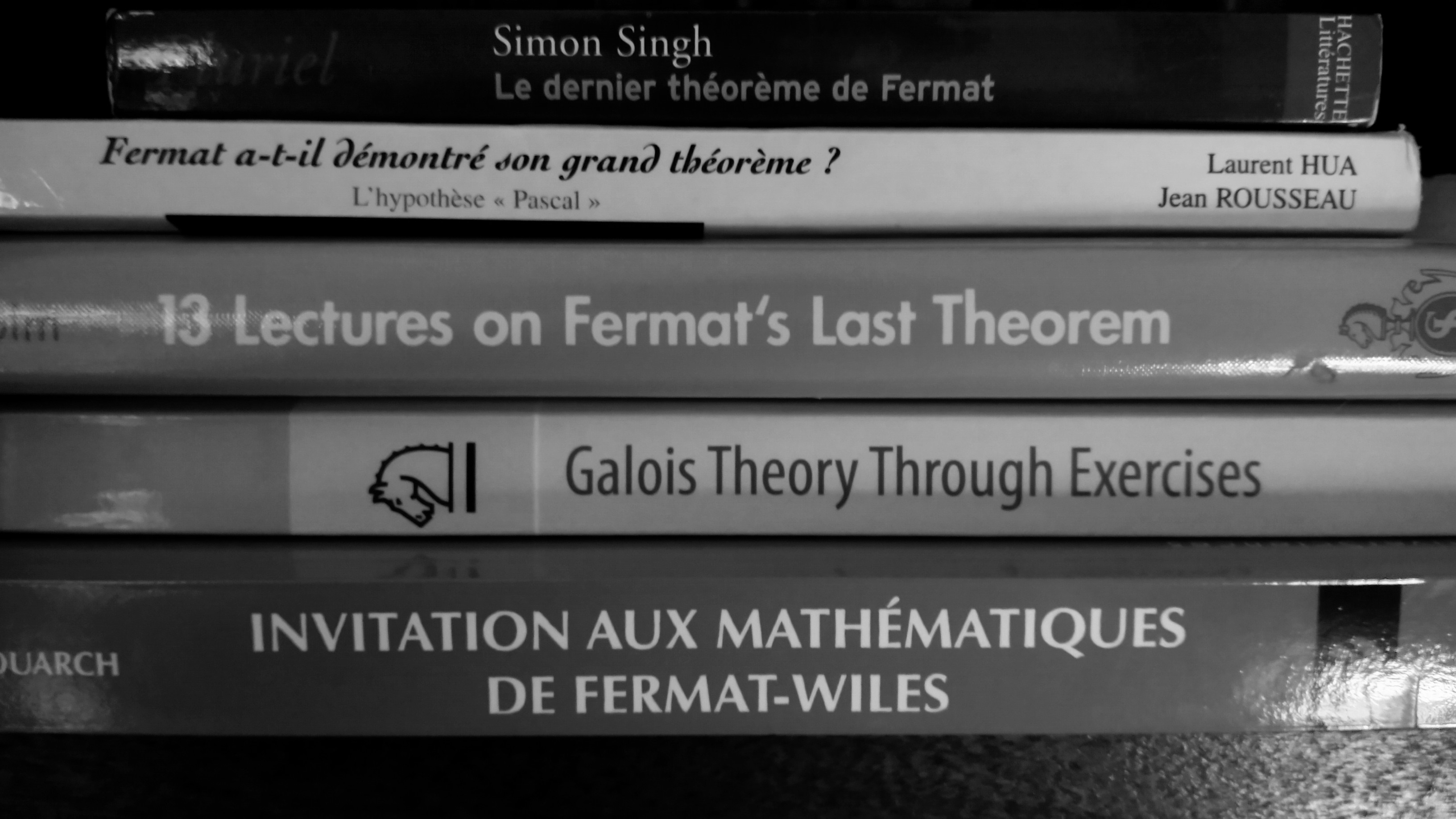
| Invitation to the Mathematics of Fermat-Wiles |
** |
Approach to Wiles proof without leaving historical approaches |
*** |
| Fermat’s Last Theorem: A Genetic Introduction to Algebraic Number Theory |
** |
Exposes the theory of algebraic integers, Kummer’s proof for regular prime and many historical details |
*** |
| Fermat’s Last Theorem for Amateurs |
* |
Many partial historical results related to FLT presented in great details. |
*** |
| 13 Lectures on Fermat’s last theorem |
** |
A lot of partial historical results related to FLT presented without details. |
** |
| Fermat a-t-il démontré son grand théorème ? L’hypothèse « Pascal » (in French) |
* |
A historical speculation around a possible proof of Fermat and a detailed analysis of his correspondance. |
** |
| Fermat last theorem |
None |
General introduction and history |
** |
| Le théorème de Fermat : son histoire by E. Nogues |
** |
A history of research around FLT, written at the beginning of the 20th century! |
* |
Details
Top 3
We can decompose the history of the main approaches of Fermat’s last theorem in three epochs: the arithmetical one (Sophie Germain, Cauchy, Legendre, Pellet…), the algebraic integers epoch (Kummer, Mirimanoff…) and the modular form (Wiles) epoch. Obviously, this misses many other approaches (sieves, analysis…) but it covers a large part of the historical publications.
These three books would cover these epochs and I strongly recommended all three of them to have a beautiful journey into the study of FLT.
Invitation to the Mathematics of Fermat-Wiles by Yves Hellegouarch
This book aims to present the proof given by Wiles. Obviously, some details will not be presented, but this is an amazing introduction. Topics presented contains introction topic (the case \(n=4\)), Kummer’s proof… Soon enough, the author jumps to Elliptic Functions, Elliptic Curves and Modular Forms which are essential.
It contains a lot of exercises and clear proofs, if there is only one book to read on the topic (and you are not afraid of mathematical details), this is probably the best one to read!
Fermat’s Last Theorem: A Genetic Introduction to Algebraic Number Theory
This one is a detailed study of Kummer’s approach. Ribenboim books only scratch the surface of this proof while here, (almost) the whole book is dedicated to give a detailed proof of Kummer’s result. Some beautiful relations between Fermat’s equation, the Zeta function and Bernoulli numbers are prestend in a very clear way, with various numeric examples. Besides, the author also dug into the archives of the French academy of science, yielding thrilling historical notes about sessions where members wrongly speculated about their possible proofs.
Fermat’s Last Theorem for Amateurs by Paulo Ribenboim
This book presents many special cases of proofs of FLT \(n=2,3,4,5,6,7...\) with many details. Though the original problem is to find solutions in the set of integers, the author propose to study this equation in other sets as well: Gaussian integers (\(\mathbb{Z}[i]\)), \(p\)-adic numbers (they truely are a hidden gem of number theory)… As the title states, it is for amateurs though this is presented as your usual math book: with theorem and proofs. Note that however, an emphasis is put on examples.
Other books
13 Lectures on Fermat’s last theorem by Paulo Ribenboim
This one is interesting: it has been written in 1979, before Fermat’s last theorem was actually proven. It summarizes many of the efforts put into trying to prove FLT and features some of the proofs. The historical context is essential, as many of the theorems are presented with notes regarding their history.
A large part of the book is devoted to the fascinating proof by Kummer and its limitations. Many other results with various importance are also presented: estimates, equivalence of FLT with other statements… One I found particularly interesting is:
- The equation \(X^{2m-1} + Y^{2m-1} = Z^{2m-1}\) has only the trivial solutions in \(\mathbb{Z}\)
- For every \(a \in \mathbb{Q}\) non-zero, the polynomial \(Z^2-a^mZ+a\) is irreducible over \(\mathbb{Q}\)
A minor regret is that many of the statements are not proved and left “as exercises” with no clue regarding their level of difficulty nor hints. It is particularly interesting to read it with Fermat’s Last Theorem for Amateurs as some of the proofs not present in this book are in the other.
However, it is remains an amazing introduction if you do not want to dig into all the details but instead are just looking for a nice overview of the history, with some details.
Fermat last theorem by Simon Singh
Requires absolutely no mathematical background. It is a very nice introduction to the problem, mostly focusing on the history of (and around) Fermat’s last theorem. Some mathematical details, along with various interesting puzzles are presented in the text and in the appendix. Really nice if you want to know what this theorem is about, and why so important it became, without digging into the mathematical details.
Fermat a-t-il démontré son grand théorème ? L’hypothèse « Pascal » (in French) by Laurent Hua and Jean Rousseau
This book is split in two parts: the first one is purely historical and does not require to know much about mathematics. The authors present the possibility that Fermat may have proved his theorem. Though the consensus seems to claim the opposite, proving than Fermat did not prove his theorem has never been done!
The first part is a thorough analysis of Fermat’s correspondance with other mathematicians of his time and it does become moving, especially towards the end. This analysis is so detailed that you even get a sense of Fermat’s sense of humor in some of the letters presented!
The second one is more mathematical, but a high school student could understand most of it. It gives what could be the starting point of a proof with the tools known by Fermat at his time. Unfortunately, it does not go too far, but the approach is interesting!
Le théorème de Fermat : son histoire by E. Nogues
Written at the beginning of the 20th century. It consists in translatiobns (in French) of all important articles regarding Fermat’s last theorem at this time. It is particularly intersting if you want to dig into the details of the history of the theorem.
In some of the books, you will need (on top of usual algebra, basic number theory and analysis tools) to know more advanced topics, such as Galois theory. To that end Galois Theory Through Exercises by Juliusz Brzeziński was my best read on this topic. It has a chapter completely dedicated to cyclotomic fields, which are an object commonly used in the books above!
Number Theory 1: Fermat’s Dream, by Kazuya Kato, Nobushige Kurokawa, Takeshi Saito this is actually the book that drove me into the study of Fermat’s Last Theorem. It is really well written, with a lot of figures, exercises and corrections.
Not read yet
The books below are my to read list. If you have any opinion on them, let me know in the comments!
Three Lectures on Fermat’s Last Theorem by Louis Joel Mordell
Mordell is a name that I now met many times! I want to read it mostly for its historical value, and to know what he had to say about this theorem, a century and a half (almost) ago!
A Course in Arithmetic by Jean-Pierre Serre
Please note that all the links above are affiliate links. However, having read these books, I am confident about the quality of my recommendations!