
A little bit of context
Quite some time ago, I asked a question on stats.stackexchange about differences between random forests and extremly random forests. Though the answers were good, I was still lacking some informations. Beyond the nice theoretical arguments, I run some simulations to have a better idea of their behavior.
Though these are, by no means, definite conclusions about their respective behaviors, those simulations performed on toy datasets, from specific implementations, I hope they will provide more insights to the reader!
Summary of the simulations
Extra trees seem much faster (about three times) than the random forest method (at, least, in scikit-learn implementation). This is consistent with the theoretical construction of the two learners.
On toy datasets, the following conclusions could be reached :
- Extra trees seem to keep a higher performance in presence of noisy features,
- When all the variables are relevant, both methods seem to achieve the same performance.
Theoretical point of view
A decision tree is usually trained by recursively splitting the data. Each split is chosen according to an information criterion which is maximized (or minimized) by one of the “splitters”. These splitter usually take the form of x[i]>t were t is a threshold and x[i] indicates the i-th component of an observation.
Decision trees, being prone to overfit, have been transformed to random forests by training many trees over various subsamples of the data (in terms of both observations and predictors used to train them).
The main difference between random forests and extra trees (usually called extreme random forests) lies in the fact that, instead of computing the locally optimal feature/split combination (for the random forest), for each feature under consideration, a random value is selected for the split (for the extra trees).
This leads to more diversified trees and less splitters to evaluate when training an extremly random forest.
The point here is not to be exhaustive, there are more references and the main articles at the bottom of the article.
Timing
First, let’s observe the timing for each model. I will use the methods implemented in scikit-learn and I will reuse a code seen in another post (the code with new minor updates is at the bottom of the post). Without a detailed analysis, it seems that Extra Trees are three times faster than the random forest method.
| N | P | Time RF | Time ET |
|---|---|---|---|
| 500 | 5 | 0.093678 | 0.0679979 |
| 500 | 10 | 0.117224 | 0.0763619 |
| 500 | 20 | 0.176268 | 0.097132 |
| 500 | 50 | 0.358183 | 0.157907 |
| 500 | 100 | 0.619386 | 0.256645 |
| 500 | 200 | 1.14059 | 0.45396 |
| 1000 | 5 | 0.139871 | 0.0846941 |
| 1000 | 10 | 0.211061 | 0.106443 |
| 1000 | 20 | 0.385125 | 0.151639 |
| 1000 | 50 | 0.805403 | 0.277682 |
| 1000 | 100 | 1.39056 | 0.501522 |
| 1000 | 200 | 2.76709 | 0.926728 |
| 2000 | 5 | 0.269487 | 0.122763 |
| 2000 | 10 | 0.474972 | 0.171372 |
| 2000 | 20 | 0.771758 | 0.264499 |
| 2000 | 50 | 1.81821 | 0.539937 |
| 2000 | 100 | 3.47868 | 1.03636 |
| 2000 | 200 | 6.95018 | 2.1839 |
| 5000 | 5 | 0.86582 | 0.246231 |
| 5000 | 10 | 1.2243 | 0.373797 |
| 5000 | 20 | 2.20815 | 0.624288 |
| 5000 | 50 | 5.13883 | 1.41648 |
| 5000 | 100 | 9.79915 | 3.25462 |
| 5000 | 200 | 21.5956 | 6.86543 |
Note the use of tabulate which allows a pretty print for python dataframes ;)
import numpy as np
import ComplexityEvaluator
from sklearn.ensemble import RandomForestRegressor, ExtraTreesRegressor, AdaBoostRegressor
from tabulate import tabulate

def random_data_regression(n, p):
    return np.random.rand(n, p), np.random.rand(n)


regression_models = [RandomForestRegressor(),
                     ExtraTreesRegressor()]

names = ["RandomForestRegressor",
         "ExtraTreesRegressor"]

complexity_evaluator = ComplexityEvaluator.ComplexityEvaluator(
    [500, 1000, 2000, 5000],
    [5, 10, 20, 50, 100, 200])

i = 0
for model in regression_models:
    res, data = complexity_evaluator.Run(model, random_data_regression)
    print(names[i])
    print tabulate(data, headers='keys', tablefmt='psql', showindex='never')
    i = i + 1
Irrelevant variables
Now, let’s try to see how they compare when we add irrelevant variables. First, we need to propose a data set where there is something to learn (as opposed as what was previously done).
Let’s fix a linear dependency between the target variable and the first three variables, along the lines of:
def linear_data_generation(n, p):
    X = np.random.rand(n, p)
    beta = np.zeros([p, 1])
    beta[0,0] = 1
    beta[1,0] = 2
    beta[2,0] = -1
    Y = np.ravel(np.dot(X, beta))
    return X, Y
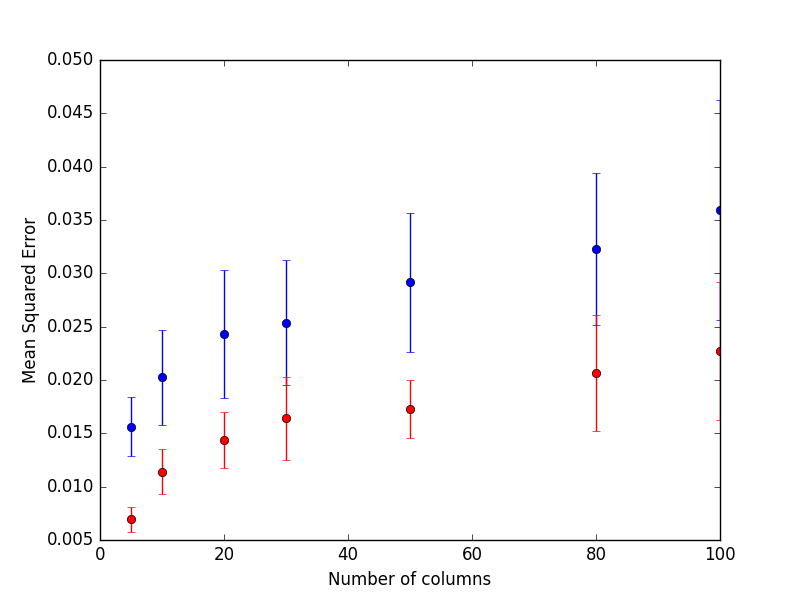
In blue are presented the results from the random forest and red for the extra trees.
The results are quite striking: Extra Trees perform consistently better when there are a few relevant predictors and many noisy ones.
import numpy as np
import AccuracyEvaluator
from sklearn.ensemble import RandomForestRegressor, ExtraTreesRegressor
from sklearn.metrics import mean_squared_error
from tabulate import tabulate
import matplotlib.pyplot as plt

def linear_data_generation(n, p):
    X = np.random.rand(n, p)
    beta = np.zeros([p, 1])
    beta[0,0] = 1
    beta[1,0] = 2
    beta[2,0] = -1
    Y = np.ravel(np.dot(X, beta))
    return X, Y


n_columns = [5, 10, 20, 30, 50, 80, 100]

accuracy_evaluator = AccuracyEvaluator.AccuracyEvaluator(
    [500],
    n_columns,
    mean_squared_error,
    10)

data_rf = accuracy_evaluator.Run(RandomForestRegressor(), linear_data_generation)
data_et = accuracy_evaluator.Run(ExtraTreesRegressor(), linear_data_generation)

plt.errorbar(n_columns, data_rf["Metric"], yerr= data_rf["Std"], fmt="o", ecolor = "blue", color="blue")
plt.errorbar(n_columns, data_et["Metric"], yerr= data_et["Std"], fmt="o", ecolor = "red", color="red")
plt.xlabel('Number of columns')
plt.ylabel('Mean Squared Error')
plt.show()
Many relevant variables
Starting from the code above and changing the decision function to be a sum of each predictor:
def linear_data_generation(n, p):
    X = np.random.rand(n, p)
    beta = np.ones([p, 1])
    Y = np.ravel(np.dot(X, beta))
    return X, Y
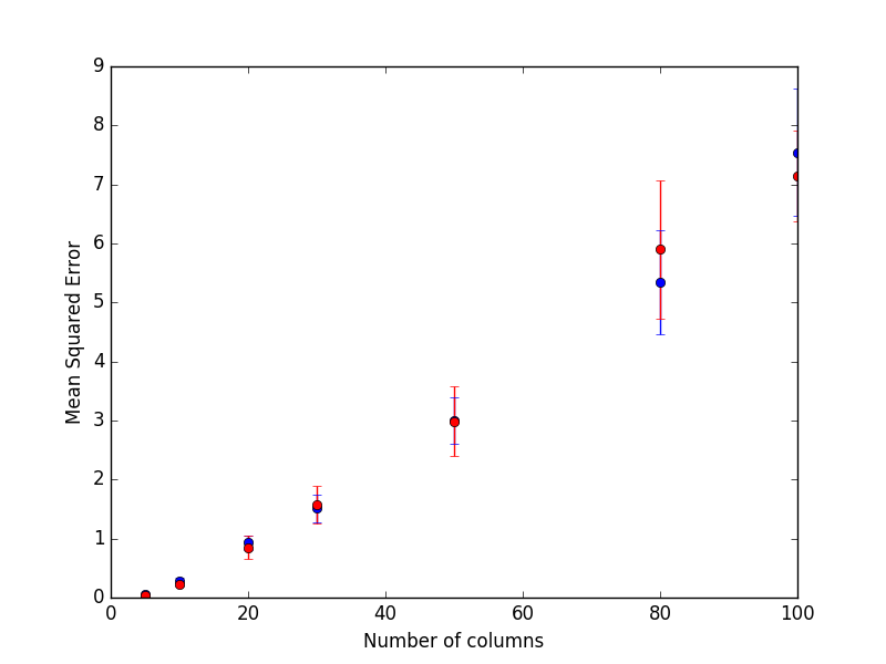
In blue are presented the results from the random forest and red for the extra trees.
It seems that both methods perform equally in presence of many relevant features.
Code
import numpy as np
import pandas as pd
import time
from sklearn.linear_model import LinearRegression
import math

class ComplexityEvaluator:

    def __init__(self, nrow_samples, ncol_samples):
        self._nrow_samples = nrow_samples
        self._ncol_samples = ncol_samples

    def _time_samples(self, model, random_data_generator):
        rows_list = []
        for nrow in self._nrow_samples:
            for ncol in self._ncol_samples:
                train, labels = random_data_generator(nrow, ncol)

                start_time = time.time()
                model.fit(train, labels)
                elapsed_time = time.time() - start_time

                result = {"N": nrow, "P": ncol, "Time": elapsed_time}
                rows_list.append(result)

        return rows_list

    def Run(self, model, random_data_generator):
        orig_data = pd.DataFrame(self._time_samples(model, random_data_generator))
        data = orig_data.applymap(math.log)
        linear_model = LinearRegression(fit_intercept=True)
        linear_model.fit(data[["N", "P"]], data[["Time"]])
        return linear_model.coef_, orig_data


if __name__ == "__main__":
    class TestModel:

        def __init__(self):
            pass

        def fit(self, x, y):
            time.sleep(x.shape[0] / 1000.)

    def random_data_generator(n, p):
        return np.random.rand(n, p), np.random.rand(n, 1)

    model = TestModel()

    complexity_evaluator = ComplexityEvaluator(
        [200, 500, 1000, 2000, 3000], [1, 5, 10])

    res = complexity_evaluator.Run(model, random_data_generator)

    print(res)
And then :
import numpy as np
import pandas as pd
import time
from sklearn.linear_model import LinearRegression
import math
from Stacker import Stacker


class AccuracyEvaluator:

    def __init__(self, nrow_samples, ncol_samples, penalty, n_folds=5):
        self._nrow_samples = nrow_samples
        self._ncol_samples = ncol_samples
        self._stacker = Stacker(penalty, n_folds, False)

    def _accuracy_samples(self, model, random_data_generator):

        def predict(model, X):
            return model.predict(X)

        rows_list = []
        for nrow in self._nrow_samples:
            for ncol in self._ncol_samples:
                train, labels = random_data_generator(nrow, ncol)

                mean_perf, std_perf,  _ = self._stacker.RunSparse(train,
                                                                  labels, model, predict)

                result = {"N": nrow, "P": ncol,
                          "Metric": mean_perf, "Std": std_perf}
                rows_list.append(result)

        return rows_list

    def Run(self, model, random_data_generator):
        orig_data = pd.DataFrame(
            self._accuracy_samples(model, random_data_generator))
        return orig_data
I will come back to stacking in another post some day, which I also use for cross-validation (stacking can be obtained almost for free during a cross validation). Plus the naming of some functions is quite unfortunate (RunSparse() should probably be called RunNumpyArray() or something like this, likewise, the Run() should probably be RunPandas()…). The code is here for the sake of completeness.
import pandas as pd
import numpy as np

from time import time
from sklearn import cross_validation


class Stacker:

    def __init__(self, penalty, n_folds, verbose=True, random_state=1):
        self._penalty = penalty
        self._n_folds = n_folds
        self._verbose = verbose
        self._random_state = random_state

    def Run(self, X, y, model, predict_method):
        kf = cross_validation.KFold(
            y.shape[0], n_folds=self._n_folds, shuffle=True, random_state=self._random_state)
        trscores, cvscores, times = [], [], []
        i = 0
        stack_train = np.zeros(len(y))  # stacked predictions
        for i, (train_fold, validation_fold) in enumerate(kf):
            i = i + 1
            t = time()
            model.fit(X.iloc[train_fold], y.iloc[train_fold])

            tr_pred = predict_method(model, X.iloc[train_fold])

            trscore = self._penalty(y.iloc[train_fold], tr_pred)

            validation_prediction = predict_method(
                model, X.iloc[validation_fold])
            cvscore = self._penalty(
                y.iloc[validation_fold], validation_prediction)

            trscores.append(trscore)
            cvscores.append(cvscore)
            times.append(time() - t)

            stack_train[validation_fold] = validation_prediction

        if self._verbose:
            print("TRAIN %.5f | TEST %.5f | TEST-STD %5f | TIME %.2fm (1-fold)" %
                  (np.mean(trscores), np.mean(cvscores), np.std(cvscores), np.mean(times) / 60))
            print(model.get_params(deep=True))
            print("\n")

        return np.mean(cvscores), stack_train

    def RunSparse(self, X, y, model, predict_method):
        kf = cross_validation.KFold(
            y.shape[0], n_folds=self._n_folds, shuffle=True, random_state=self._random_state)
        trscores, cvscores, times = [], [], []
        i = 0
        stack_train = np.zeros(len(y))  # stacked predictions
        for i, (train_fold, validation_fold) in enumerate(kf):
            i = i + 1
            t = time()
            model.fit(X[train_fold], y[train_fold])

            tr_pred = predict_method(model, X[train_fold])

            trscore = self._penalty(y[train_fold], tr_pred)

            validation_prediction = predict_method(
                model, X[validation_fold])
            cvscore = self._penalty(
                y[validation_fold], validation_prediction)

            trscores.append(trscore)
            cvscores.append(cvscore)
            times.append(time() - t)

            stack_train[validation_fold] = validation_prediction

        if self._verbose:
            print("TRAIN %.5f | TEST %.5f | TEST-STD %5f | TIME %.2fm (1-fold)" %
                  (np.mean(trscores), np.mean(cvscores), np.std(cvscores), np.mean(times) / 60))
            print(model.get_params(deep=True))
            print("\n")

        return np.mean(cvscores), np.std(cvscores),stack_train
Learning more and references
The elements of statistical learning by Trevor Hastie, Robert Tibshirani, Jerome Friedman is a brilliant introduction to the topic and will help you have a better understanding of most of the algorithms presented in this article !
Classification and Regression Trees by Leo Breiman, Jerome Friedman, Charles J. Stone, R.A. Olshen
Breiman L (2001). “Random Forests”. Machine Learning. 45 (1): 5–32.
Geurts P, Ernst D, Wehenkel L (2006). “Extremely randomized trees”. Machine Learning. 63: 3–42
Python data science handbook