As an occasionnal “Kaggler” I like to write my own code or experiment new alogrithms. This one led me to a top 20 place. The solution was really simple: each line of the train and test set is described as a collection of binary feature. For each feature, one can associate the destinations who share this feature. If the cloud of points associated to this binary feature has a low “variance” (i.e. most of the points sharing this feature end up in the same place) and a high number of observations, we want to give a higher weight to this feature. Otherwise, this feature can be deemed as poorly informative and we want to decrease its weight.
Preprocessing
-
Generate a set of balls covering the map (radiuses and centers being chosen to avoid having too many features in the end)
-
Remove the trajectories with lightspeed jumps
-
For the training, cut the trajectories according to a \(\min(U[0,1],U[0,1])\) law (it provided a good matching between cross validation and leaderboard score).
-
Replace the (truncated) trajectories by the set of balls they cross
-
Keep all the other features
Learning
-
For each feature (boolean: have this trajectory crossed Ball k, is it id_207?) generate a cloud of points that are the final points sharing this feature. Actually, the cloud itself is never stored in memory (it would not fit on most computers I guess). Only its barycentre and variance are (they are then updated as mean and variance would be).
-
Features and their interactions were considered. Indeed, without interactions the performance is really low. Interactions such as “Is the car on the road to the airport AND is the car going north” intuitively seem much more efficient than the two features taken independently.
Predicting
-
Given the features, gather all the barycenters and variances.
-
Return an average of the barycenters, weighted by the inverse of the standard deviation (raised to a certain power - CV showed that 7 was the best) :
- \[\hat{f}(p_{1}...p_{n})=\sum_{k,p_{k}\,is\,true}\frac{\#\left(C\left(p_{k}\right)\right)^{\alpha}\mathrm{bar}(C(p_{k}))}{\mathrm{sd}\left(C(p_{k})\right)^{\beta}}\]
Where :
\(p_{k}\) stands for a boolean feature,
\(C(p_{k})\) stands for the cloud associated to the feature,
\(\#\left(C(p_{k})\right)\), sd and bar stands for the number of points, the variance and the barycenter of the cloud.
\(\alpha\) and \(\beta\) are penalization parameters.
Speed of the algorithm
Using streaming evaluation of mean and standard deviation of a collection of points, this algorithms had a linear complexity in terms of the number of points. The training and testing part could actually be performed in a couple of minutes.
How to improve it ?
Performance
Considering interactions of depth 3 ! Unfortunatly, I was limited by my computer’s memory.
Combining this with other approaches (genuine random forests…) could have helped as well!
Speed
The part:
Generate a set of balls covering the map (radiuses and centers being chosen to avoid having too many features in the end)
Could actually have been made much faster using squares (and rounding) insteads of balls! The algorithm with balls had a \(O(n \cdot d)\) complexity (\(d\) being the number of balls) whereas rounding would have led to a \(O(n)\) complexity, no matter the number of squares.
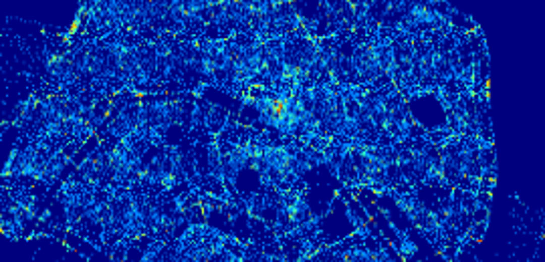
Bonus: generating heatmaps!
The data comes from OpenData.Paris.fr and is inspired from the following kernel.
import numpy as np
import pandas as pd
import matplotlib.pyplot as plt

bins = 500
lat_min, lat_max = 48.75, 48.95
lon_min, lon_max = 2.25, 2.5

COLNAME = "Geometry X Y"

def getCoord(x,i):
    return map(float, x.split(','))[i]


data = pd.read_csv("./troncon_voie.csv",
                   chunksize=10000,
                   usecols=[COLNAME],
                   sep=";")

z = np.zeros((bins, bins))

for i, chunk in enumerate(data):
    print("Chunk " + str(i))
    chunk['x'] =chunk[COLNAME].apply(lambda x: getCoord(x,0))
    chunk['y'] =chunk[COLNAME].apply(lambda x: getCoord(x,1))
    z += np.histogram2d(chunk['x'], chunk['y'], bins=bins,
                        range=[[lat_min, lat_max],
                               [lon_min, lon_max]])[0]

log_density = np.log(1 + z)

plt.imshow(log_density[::-1, :],  # flip vertically
           extent=[lat_min, lat_max, lon_min, lon_max])


plt.savefig('heatmap.png')