
Too long, didn’t read
General remarks
If you have too many rows (more than 10 000), prefer the random forest. If you do not have much time to pre process the data (and, or have a mix of categorical and numerical features), prefer the random forest.
Classification tasks
Random forests are inherently mutliclass whereas Support Vector Machines need workarounds to treat multiple classes classification tasks. Usually this consists in building binary classifiers which distinguish (i) between one of the labels and the rest (one-versus-all) or (ii) between every pair of classes (one-versus-one).
Empiric facts
Do we Need Hundreds of Classifiers to Solve Real World Classification Problems?
This article is a must read. The authors run 179 classification algorithms over 121 datasets. One of their conclusion being:
The classifiers most likely to be the bests are the random forest (RF) versions, the best of which (implemented in R and accessed via caret)
For the sake of the example, the next two paragraphs deal with datasets where SVMs are better than random forests.
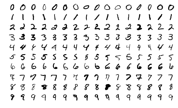
MNIST benchmark
From crossvalidated, RFs seem to achieve a 2.8% error rate on the MNSIT dataset.
On the other hand, on Yann Lecun benchmarks a simple SVM with a gaussian kernel could reach a 1.4% error rate. Virtual SVM could reach 0.56% error rate.
Microarray data
Quoting A comprehensive comparison of random forests and support vector machines for microarray-based cancer classification, who use 22 diagnostic and prognostic datasets:
We found that both on average and in the majority of microarray datasets, random forests are outperformed by support vector machines both in the settings when no gene selection is performed and when several popular gene selection methods are used.
Size of the data set and theoretical complexity
The first thing to consider is the feasability of training a model on a specific data set. Are there too many rows or columns to train a specific model ? Recall the table from the article about time complexity.
| Algorithm | Classification/Regression | Training | Prediction |
|---|---|---|---|
| Decision Tree | C+R | \(O(n^2p)\) | \(O(p)\) |
| Random Forest | C+R | \(O(n^2pn_{trees})\) | \(O(pn_{trees})\) |
| Random Forest | R Breiman implementation | \(O(n^2p n_{trees})\) | \(O(pn_{trees})\) |
| Random Forest | C Breiman implementation | \(O(n^2 \sqrt p n_{trees})\) | \(O(pn_{trees})\) |
| SVM (Kernel) | C+R | \(O(n^2p+n^3)\) | \(O(n_{sv}p)\) |
What we can see is that the computational complexity of Support Vector Machines (SVM) is much higher than for Random Forests (RF). This means that training a SVM will be longer to train than a RF when the size of the training data is higher.
This has to be considered when chosing the algorithm. Typically, SVMs tend to become unusable when the number of rows exceeds 20 000.
Therefore, random forests should be prefered when the data set grows larger. You can use, however, bagged support vector machines.
Transformation of the data : practical details
Recall the following table, which can be found in the article about data scaling and reducing
| Algorithm | Translation invariant | Monotonic transformation invariant |
|---|---|---|
| Decision Tree | X | X |
| Random Forest | X | X |
| Gradient Boosting | X | X |
| SVM (Gaussian kernel) | X | |
| SVM (Other kernels) |
This simply means that you do not have to worry about scaling / centering data or any other transformation (such as Box Cox) before feeding your data to the random forest algorithm.
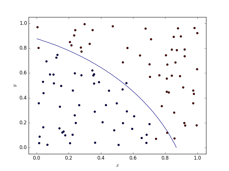
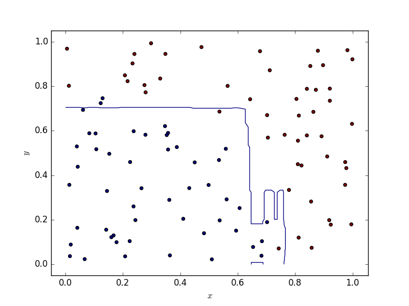
The shape of the decision function
One scarcely has to deal with two dimensional data. If this ever happens to you, bear in mind that random forest tend to produce decision boundaries which are segements parallel to the x and y axises, whereas SVMs (depending on the kernel) provide smoother boundaries. Below are some illustrations.
Results
The code
import numpy as np
from sklearn.ensemble import RandomForestClassifier, ExtraTreesClassifier, AdaBoostClassifier
from sklearn.svm import SVR, SVC
from sklearn.neighbors import KNeighborsClassifier
from sklearn.linear_model import LogisticRegression
from DecisionBoundaryPlotter import DecisionBoundaryPlotter


def random_data_classification(n, p, f):
    predictors = np.random.rand(n, p)
    return predictors, np.apply_along_axis(f, 1, predictors)


def parabolic(x, y):
    return (x**2 + y**3 > 0.5) * 1


def parabolic_mat(x):
    return parabolic(x[0], x[1])


X, Y = random_data_classification(100, 2, parabolic_mat)

dbp = DecisionBoundaryPlotter(X, Y)

named_classifiers = [(RandomForestClassifier(), "RandomForestClassifier"),
                     (SVC(probability=True), "SVC")]

for named_classifier in named_classifiers:
    print(named_classifier[1])
    dbp.PlotContour(named_classifier[0], named_classifier[1])
    dbp.PlotHeatmap(named_classifier[0], named_classifier[1])
The DecisionBoundaryPlotter class being defined below:
import numpy as np
import matplotlib.pyplot as plt


class DecisionBoundaryPlotter:

    def __init__(self, X, Y, xs=np.linspace(0, 1, 100),
                 ys=np.linspace(0, 1, 100)):
        self._X = X
        self._Y = Y
        self._xs = xs
        self._ys = ys

    def _predictor(self, model):
        model.fit(self._X, self._Y)
        return (lambda x: model.predict_proba(x.reshape(1,-1))[0, 0])

    def _evaluate_height(self, f):
        fun_map = np.empty((self._xs.size, self._ys.size))
        for i in range(self._xs.size):
            for j in range(self._ys.size):
                v = f(
                    np.array([self._xs[i], self._ys[j]]))
                fun_map[i, j] = v
        return fun_map

    def PlotHeatmap(self, model, name):
        f = self._predictor(model)
        fun_map = self._evaluate_height(f)

        fig = plt.figure()
        s = fig.add_subplot(1, 1, 1, xlabel='$x$', ylabel='$y$')
        im = s.imshow(
            fun_map,
            extent=(self._ys[0], self._ys[-1], self._xs[0], self._xs[-1]),
            origin='lower')
        fig.colorbar(im)
        fig.savefig(name + '_Heatmap.png')

    def PlotContour(self, model, name):
        f = self._predictor(model)
        fun_map = self._evaluate_height(f)

        fig = plt.figure()
        s = fig.add_subplot(1, 1, 1, xlabel='$x$', ylabel='$y$')
        s.contour(self._xs, self._ys, fun_map, levels = [0.5])
        s.scatter(self._X[:,0], self._X[:,1], c = self._Y)
        fig.savefig(name + '_Contour.png')
SVM as a random forest
Something funny is that random forests can actually be rewritten as kernel methods. I have not (yet) looked at the articles below in more details
Random forests and kernel methods, Erwan Scornet
The Random Forest Kernel (and creating other kernels for big data from random partitions)
Towards faster SVMs ?
As I was writing the article, I discovered some recent progresses had been made : a scalable version of the Bayesian SVM has been developed. See : Bayesian Nonlinear Support Vector Machines for Big Data.
Learning more
Wenzel, Florian; Galy-Fajou, Theo; Deutsch, Matthäus; Kloft, Marius (2017). “Bayesian Nonlinear Support Vector Machines for Big Data”. Machine Learning and Knowledge Discovery in Databases (ECML PKDD).
The elements of statistical learning by Trevor Hastie, Robert Tibshirani, Jerome Friedman is a brilliant introduction to the topic and will help you have a better understanding of most of the algorithms presented in this article !
Classification and Regression Trees by Leo Breiman, Jerome Friedman, Charles J. Stone, R.A. Olshen