There are plenty of tutorials here and there to have Python and vim interact beautifully. The point of this one is to provide some simple lines to add to you .vimrc file without to worry too much about installing more (vim) packages. Having myself struggled to implement this line, I will provide some explanations about the meaning of each of them.

If you have more tricks for your common datascience tasks in vim, let me know, I will add them!

Introduction

Summary

Here are the thing you can do with the following settings:

• Associate the common import to keypresses,
• Preview the contents of a csv file in a vim pane,
• Format JSON files with jq or python files with autopep8,
• Quickly add print() statements,
• Fix the usual copy paste into vim (bonus).

If you are familiar with vim, you will know that you can do pretty much everything with a sequence of keypresses. Recording this keypresses and mapping them to another key just factors everything you want to do ;)

Requirements

Python packages: pandas, autopep8, numpy Packages: jq.

Data preview

I start with the hardest but most satisfying command:

autocmd FileType python map <C-F9> va"y:!python -c "import pandas as pd; df=pd.read_csv('<C-R>"', nrows=5); print(df)" > tmp.tmp<CR>:sv tmp.tmp<CR>:resize 8<CR>

It will show the first five lines of the .csv file in the quotes surrounding the cursor in a new vim pane.

Details

autocmd FileType python is just saying that the mapping which follows will only apply to python files. This avoids accidental application to other languages.

map <C-F9> means map Ctrl + F9 to the following sequence of keypresses

va"y is a way to tell vim :

• select v

• around a

• quotes "

• copy y (to register)

:! allows to execute vim commands in your actual terminal

python -c "import pandas as pd; df=pd.read_csv('<C-R>"', nrows=5); print(df)" now we are doing one line python, the only trick here is the <C-R> which refers to vim clipboard (or register), so what we stored when “pressing” va"y.

> tmp.tmp<CR>:sv tmp.tmp<CR>:resize 8<CR> outputs the Python print statement to a tmp file (tmp.tmp) which in turn is opened by vim (with :sv)

Beautifying files

Python

This one needs autopep8 installed. Otherwise, it will just remove everything in the file you are editing…

autocmd FileType python map <F4> :!autopep8 --in-place --aggressive %<CR>

It will format your Python scripts using the autopep8 guidelines.

JSON

This one needs to have jq installed. It is a tool to manipulate JSON files easily and I strongly recommend using it.

autocmd FileType json map <F4> :%! jq .<CR>

Upon pressing <F4> it will ident your file beautifully.

Python

Execution

If I want to execute quickly the script I am working on, these two lines enable to do it (whether I am in visual or edit mode)

autocmd FileType python map <F5> :wall!<CR>:!python %<CR>
autocmd FileType python imap <F5> <Esc>:wall!<CR>:!python %<CR>

It is ideal when you are used to test your classes like this:

from collections import defaultdict

class MarkovLikelihood:

    def __init__(self, alpha):
        self.alpha_ = alpha
        self.transition_counts_ = defaultdict(lambda: 0)
        self.start_counts = defaultdict(lambda: 1)

    def fit(self, sentences):
        for sentence in sentences:
            self.update_(sentence)
        return self
    
    def update_(self, sentence):
        words = sentence.split(' ')
        for w1, w2 in self.pairwise_(words):
            self.transition_counts_[f"{w1}_{w2}"] += 1
            self.start_counts[w1] += 1

    def pairwise_(self, iterable):
        a = iter(iterable)
        return zip(a, a)

    def predict(self, sentence):
        res = 1
        words = sentence.split(' ')
        n = len(words)
        for w1, w2 in self.pairwise_(words):
            res *= (self.transition_counts_[f"{w1}_{w2}"] + self.alpha_) / self.start_counts[w1]

        return res
    
if __name__ == "__main__":


    ml = MarkovLikelihood(0.5)
    sentences = [ 
        "I ate dinner.",
        "We had a three-course meal.",
        "Brad came to dinner with us.",
        "He loves fish tacos.",
        "In the end, we all felt like we ate too much.",
        "We all agreed; it was a magnificent evening."]

    ml.fit(sentences)

    res = ml.predict("dinner with tacos")
    print(res)
    res = ml.predict("I love tennis")
    print(res)

Imports

The following two lines allow to have the most common imports with a couple of keypresses:

autocmd FileType python map <C-F10> ggiimport pandas as pd<CR>import numpy as np<CR>np.random.seed(0)<CR><Esc>
autocmd FileType python map <C-F11> ggiimport matplotlib.pyplot as plt<CR>import seaborn as sns<CR><Esc>

Will add the following to the Python file you are working on. Note that gg makes sure to place the cursor at the top of the file first.

import matplotlib.pyplot as plt
import seaborn as sns
import pandas as pd
import numpy as np
np.random.seed(0)

Quick print

autocmd FileType python map <C-p> viwyoprint(<Esc>pA)<Esc>

if your cursor is on a word (my_variable), it will simply append a print(my_variable) statement below the current line. Useful for debugging.

Fixing copy and paste

" Automatically set paste mode in Vim when pasting in insert mode
" https://coderwall.com/p/if9mda/automatically-set-paste-mode-in-vim-when-pasting-in-insert-mode
let &t_SI .= "\<Esc>[?2004h"
let &t_EI .= "\<Esc>[?2004l"

inoremap <special> <expr> <Esc>[200~ XTermPasteBegin()

function! XTermPasteBegin()
  set pastetoggle=<Esc>[201~
  set paste
    return ""
endfunction

Introduction

A not so famous algorithm

Regularized Greedy Forest is a quite recent algorithm in machine learning, the article “Learning Nonlinear Functions Using Regularized Greedy Forest” has been published in 2014.

If we want to compare it to gradient boosting, which seems to have been studied back in 1999, it took a while before this algorithm received its many reliable and fast implementations (xgboost, catboost, LightGBM).

It seems to be a very good candidate in terms of performance. However, as we will see in the parameters section, it requires some tuning (regularization and number of leaves can be application critical).

Performance

As stated by the authors, Regularized Greedy Forest can achieve better performance than gradient boosting approaches:

In contrast to these traditional boosting algorithms that treat a tree learner as a black box, the method we propose directly learns decision forests via fully-corrective regularized greedy search using the underlying forest structure. Our method achieves higher accuracy and smaller models than gradient boosting on many of the datasets we have tested on.

And if you are skeptical about benchmarks proposed by the authors, check out the following posts, related to data science competitions:

• 1st Place Solution (TReNDS Neuroimaging)
• 1st Place Solution (Home Credit Default Risk)
• 1st Place Solution (Allstate Claims Severity)
• 2nd Place Solution (Home Credit Default Risk)
• 3rd Place Solution (Santander Customer Satisfaction)
• 13th Place Solution (IEEE-CIS Fraud Detection)
• 18th Place Solution (Porto Seguro’s Safe Driver Prediction)
• 35th Place Solution (Porto Seguro’s Safe Driver Prediction)
• Kernel (Porto Seguro’s Safe Driver Prediction)

On top of that, I noted that on some dataset I have comparable performance between xgboost and RGF after a careful tuning of the parameters for both the models.

How does it work ?

The algorithm

As for gradient boosting and random forests, the idea is to train a collection of decision trees. However, the key difference is that you are allowed to modify previously trained trees and weights attributed to each tree if that improves the performance of the overall model.

To make things more clear:

• In the case of random forests, all the trees are trained simultaneously and regardless of each other performance.
• In the case of gradient boosting, a new tree is trained on the residuals of the previous trees.
• In the case of random greedy forest, things are more complicated :) At each step we may either start a new tree, or split an existing leaf node. Then, the weights of each leaf are adjusted, to optimize the loss function.

To put it in equations, when we try to learn some objective function \(F\) what we do is to solve this type of optimization program.

The space of functions where \(F\) lives being quite large, we usually rely on heuristics to make the above problem solvable in an acceptable amount of time.

Per example, in the case of gradient boosting, we solve a series of training of decision trees, with the following induction:

\(F_m(x) = F_{m-1}(x) + \underset{h_m \in \mathcal{H}}{\operatorname{arg\,min}} \left[{\sum_{i=1}^n {L(y_i, F_{m-1}(x_i) + h_m(x_i))}}\right]\),

So that each step is as simple as training a decision tree, and the training time is, roughly, the number of trees times the training time of a tree.

In the case of the Regularized Greedy Forest, the procedure is as follows:

• Fix the weights, and change the structure of the forest (which changes basis functions) so that the loss $Q(F)$ is reduced the most.
• Fix the structure of the forest, and change the weights so that lossQ(F) is minimized

Cross validating a random greedy forest

The cross validation is usual, here are the roles of the different parameters.

Parameters description

The parameters are sorted by order of importance in terms of their impact on the accuracy of the model.

max_leaf : the total number of leaves in the forest. Note that given the training procedure, we never have to specify the total number of trees needed in the forest. Beware, the larger this parameter, the longer the training. By default, the value is 1000 for RGFClassifier and 500 RGFRegressor.

l2 : the penalty. This parameter has to be tuned to obtain a good performance. By default, the value is 0.1 but smaller values usually improve performance.

n_tree_search : (1 by default) Number of trees to be searched for the nodes to split.

algorithm one of (“RGF”, “RGF_Opt”, “RGF_Sib”), where the algorithm are the following:

• RGF: RGF with L2 regularization on leaf-only models.
• RGF Opt: RGF with min-penalty regularization.
• RGF Sib: RGF with min-penalty regularization with the sum-to-zero sibling constraints.

By default, the algorithm is “RGF” for both RGFClassifier() and RGFRegressor().

reg_depth : Must be no smaller than 1.0. Meant for being used with algorithm="RGF_Opt"|"RGF_Sib". A larger value penalizes deeper nodes more severely.

loss one of ("LS", "Expo", "Log", "Abs"), by default this is LS for regressions and Log for classification.

• LS: Square loss,
• Expo: Exponential loss,
• Log: Logistic loss,
• Abs: Absolute error loss.

n_iter : Number of iterations of coordinate descent to optimize weights. If None, 10 is used for loss=”LS” and 5 for loss=”Expo” or “Log”. Not critical to improve accuracy.

Classification only

calc_prob : One of (“sigmoid”, “softmax”), by default “sigmoid”. I guess it will not affect accuracy or roc_auc, but may affect logloss.

Benchmarks

Code

Fortunately, the implementation comes with a scikit learn interface, therefore you can use the usual .fit() and .transform() methods, so there is not much to say about how to use it. Per example, the following will cross validate a random greedy forest.

from sklearn import datasets
from sklearn.utils.validation import check_random_state
from sklearn.model_selection import StratifiedKFold, cross_val_score
from rgf.sklearn import RGFClassifier

iris = datasets.load_iris()
rng = check_random_state(0)
perm = rng.permutation(iris.target.size)
iris.data = iris.data[perm]
iris.target = iris.target[perm]

rgf = RGFClassifier(max_leaf=400,
                    algorithm="RGF_Sib",
                    test_interval=100,
                    verbose=True)

n_folds = 3

rgf_scores = cross_val_score(rgf,
                             iris.data,
                             iris.target,
                             cv=StratifiedKFold(n_folds))

rgf_score = sum(rgf_scores)/n_folds
print('RGF Classifier score: {0:.5f}'.format(rgf_score))

References

Learning Nonlinear Functions Using Regularized Greedy Forest is the main article on the topic.

The RGF implementation for the basic implementation, and for the sparse implementation (FastRGF).

What is overfit ?

Overfit is somehow what happens when you “train your model too much”. In that case, you achieve a very good training accuracy, while the test accuracy is usually poor. Think about a one dimensional regression. You may either fit a straight line, or draw a line that passes through every point. Which one will generalize best ?

In the cases of some models, there are some specific parameters that can control the balance between “passing through every point” and “drawing a straight line”. In the case of gradient boosting, this will be the number of trees, in the case of neural networks, it will be the number of iterations in the gradient descent, in the case of support vector machines, a combination of parameters…

A quite common figure regarding overfit is the following:

It applies mostly to neural network, where the abscissa represents the number of epochs, the blue line the training loss and the red line the validation loss.

The same question applies to gradient boosting, where the number of trees if quite critical and could replace the abscissa on the upper graph, see per example this question. Some people seem to claim that it should not overfit (as random forest do not overfit).

Simulations

A cool python library

While looking for bencharmk data, I found pmlb which stands for Penn Machine Learning Benchmark. Basically it enables to download different real word datasets.

More info can be found in the project page.

Method

I used xgboost for which I simply increased the number of trees.

for n_trees in [10, 20, 50, 100, 200, 1000, 1500, 2000, 3000, 4000, 10000, 30000]:
    for max_depth in [5]:
        for learning_rate in [0.001]:
            yield {
                    "name": "XGBClassifier",
                    "parameters": {
                        "n_estimators": n_trees,
                        "max_depth": max_depth,
                        "learning_rate": learning_rate,
                        }
              }

On the following datasets:

['heart_statlog', 'hepatitis', 'horse_colic', 'house_votes_84', 'hungarian', 'hypothyroid', 'ionosphere', 'iris', 'irish', 'kr_vs_kp', 'krkopt', 'labor', 'led24', 'led7', 'letter', 'lupus', 'lymphography', 'magic']

The performance of each model was then evaluated using a 5 folds cross validation for the following metrics ["roc_auc", "accuracy", "neg_log_loss"].

Does xgboost overfit ?

The graphs below seem to say that increasing the number of trees may harm the performance of the model. However, in some cases, even very large number of trees are beneficial to the model.

Graphs

Comparison with random forest

However, the comparison with random forests is needed to understand what was at stake above:

Code

from pmlb import fetch_data
import pandas as pd
import numpy as np
from sklearn.model_selection import cross_validate
from model_builder import model_builder


def run(model_parameters, dataset_key, metrics):
    model = model_builder(model_parameters)
    X, y = fetch_data(dataset_key, return_X_y=True)
    if len(np.unique(y)) != 2:
        print("Problem is not binary")
        return None

    res = cross_validate(model, X, y, scoring=metrics)

    row = {
            "fit_time": np.mean(res["fit_time"]),
            "n": X.shape[0],
            "p": X.shape[1]
            }
    for metric in metrics:
        row[metric] = np.mean(res[f"test_{metric}"])
        row[f"{metric}_std"] = np.std(res[f"test_{metric}"])
    return row


def benchmark():

    for n_trees in [10, 20, 50, 100, 200, 1000, 1500, 2000, 3000, 4000, 10000, 30000]:
        for max_depth in [5]:
            for learning_rate in [0.001]:
                yield {
                        "name": "XGBClassifier",
                        "parameters": {
                            "n_estimators": n_trees,
                            "max_depth": max_depth,
                            "learning_rate": learning_rate,
                            }
                    }

dataset_keys = ['heart_statlog', 'hepatitis', 'horse_colic', 'house_votes_84', 'hungarian', 'hypothyroid', 'ionosphere', 'iris', 'irish', 'kr_vs_kp', 'krkopt', 'labor', 'led24', 'led7', 'letter', 'lupus', 'lymphography', 'magic']
rows = []

for dataset_key in dataset_keys:
    for model in benchmark():
        row = run(model, dataset_key, ["roc_auc", "accuracy", "neg_log_loss"])
        if row is not None:
            row["model"] = model["name"]
            row["data"] = dataset_key
            row = {**row, **model["parameters"]}
            print(row)
            rows.append(row)

output_data = pd.DataFrame(rows)
output_data.to_csv("./xgb_overfit.csv", index=False)

And the graphs can be produced easily using the nice .plot() methods proposed by pandas and matplotlib.

import pandas as pd
import matplotlib.pyplot as plt

for metric in ["roc_auc", "accuracy", "neg_log_loss"]:
    benchmark_data = pd.read_csv("xgb_overfit.csv")
    benchmark_data.set_index("n_estimators", inplace=True)
    benchmark_data.groupby("data")[metric].plot(legend=True, logx=True, title=metric)
    plt.legend(loc="lower left")
    plt.savefig(f"xgb_{metric}.svg")
    plt.clf()

References

• xgboost one of the best gradient boostin libraries available.

• pmlb a Python library providing various benchmark datasets.

Keras memory usage keeps increasing

I was having fun, attempting to do some deep learning with a 2M lines dataset (nothing my computer can’t handle, xgboost was running with roughly 15% of my RAM) when suddenly, as I was adding neural networks in my fancy stacked models, the script kept failing, the memory usage went to the moon, etc, etc.

What did I do wrong ? Did I introduce a memory leak between my model stacking / neural network factory code ? I would be suprised, it worked fine with every other model. And a neural network is more or less a simple vector of floats (in my case, with only hundreds of parameters) so there is no reason for it to be that big.

The only thing I was attempting to do was to cross validate different neural networks, with different architectures.

So, after a quick research : I found this stack overflow question , also some people mentioning a weird behavior coming from model.predict() . Another Github issue is simply called Memory leak . There even is another article simply titled Dealing with memory leak issue in Keras model training and is even mentioned on twitter .

What I ended up suspecting is that there are actually many memory leaks from different methods in the code. So I gathered the list of workarounds I could find.

Workarounds

Beware, none of them actually works. Some just alleviate the pain, but most likely, the memory usage will keep increasing. Anyways, the good news is that, combining many of the tricks I could read, I managed to have my models run ;)

Garbage collecting

Generally, when you see these lines in the code it means that the person who wrote it was desperate to make it run while closely monitoring the memory usage of the script and combined tricks not to make sure everything was fitting into the memory. Usually, performing tasks in dedicated functions and trusting the garbage collector to do its job at the right time is enough. But sometimes you meet these del / garbage collector random invokations.

import gc
del model
gc.collect()
K.clear_session()

I did put these lines after every model.fit() I found. They did not help at all in my case.

Force eager evaluation

This one kind of worked for me. It slows down the training (3 times slower in my case), the memory keeps increasing for no reason, but much less. Just add the following argument in the model.compile() method :

model.compile( [...]
              run_eagerly=True)

model(x) instead of model.predict(x)

Some people mentioned it. It did not change a thing for me, but I wrote it that way. Be careful though, model(x) will return a tensorflow object while model.predict(x) will return a numpy object.

Run it in a dedicated script

Yes, kind of ugly. It does not solve the issue, but if you make your cross validation in a python script, itself being called from the terminal level, you can pass parameters using JSON and hope that each script won’t hit your memory limit.

In my case, I wrote the following class:

from tensorflow.keras.layers import Dense
from tensorflow.keras.models import Sequential
import tensorflow as tf
import gc
import numpy as np

class NNModel:

    def __init__(self, architecture, epochs, loss="binary_crossentropy", optimizer="adam"):
        self._epochs = epochs
        self._loss = loss
        self._optimizer = optimizer
        self._architecture = architecture
        self._model = None

    def fit(self, X, y):

        gc.collect()
        tf.keras.backend.clear_session()
    
        self._model = self._model_factory(X.shape[1])

        X_tf = tf.convert_to_tensor(X, dtype=tf.float32)
        y_tf = tf.convert_to_tensor(y, dtype=tf.float32)

        self._model.fit(X_tf, y_tf, epochs=self._epochs)
        return self

    def _model_factory(self, input_dim):

        model = Sequential()

        architecture = self._architecture.copy()
        first_layer = architecture.pop(0)

        model.add(Dense(first_layer[0], input_dim=input_dim, activation=first_layer[1]))
        for layer in architecture:
            model.add(Dense(layer[0], activation=layer[1]))

        model.compile(loss=self._loss, 
                      optimizer=self._optimizer, 
                      run_eagerly=True,
                      metrics=['accuracy'])

        return model

    def predict(self, X):
        raise NotImplementedError

    def predict_proba(self, X):
        X_tf = tf.convert_to_tensor(X, dtype=tf.float32)
        res =  self._model(X_tf)
        res = np.hstack((1-res, res))
        return res

Which I can configure using a JSON that will contain the arguments of the class constructor:

{
  "epochs": 8,
  "architecture": [[ 12, "relu" ], [ 8, "relu" ], [ 1, "sigmoid" ]]
}

And then I invoke them with:

find ../models/ -name \*.json | xargs --max-args=1 python run_nn.py

So that I can run my different models while I am sure that the memory will be totally released between the execution of two scripts.

model.predict_on_batch

Quoting MProx from a git issue

I have managed to get around this error by using model.predict_on_batch() instead of model.predict(). This returns an object of type <class ‘tensorflow.python.framework.ops.EagerTensor’> - not a numpy array as claimed in the docs - but it can be cast by calling np.array(model.predict_on_batch(input_data)) to get the output I want.

Side note: I also noticed a similar memory leak problem with calling model.fit() in a loop, albeit with a slower memory accumulation, but this can be fixed in a similar way using model.train_on_batch().

I did not try this one, as segregating different models in different scripts and setting run_eagerly did the job.

Less recommended approaches

Use tf-nightly

So, tf-nightly is built more or less every day, with the latest features and less tests. Many people claimed that the leak disapeared when using this library. But there are many versions, with potentially other bugs.

re install the 1.14 version

This bug has been around for a while, some tickets mention it from october 2019 and it is still present in the 2.4 version.

Conclusion

I look forward to this issue being solved.

As far as I know, there is no implementation of argmax and argmin in the default ocaml library (or perhaps they could be called maxi for more consistency with respect to mapi). The following snippet solves it!

let argmax l =
  let rec aux max_index index max_value = function
    | [] -> max_index
    | h::t -> if h > max_value then aux index (index + 1) h t 
                         else aux max_index (index + 1) max_value t
  in 

  match l with 
  | [] -> 0
  | _ ->   aux 0 0 (List.hd l) l

Note that the defaut behavior with an empty list is to return 0 but it can be changed.

Taking screenshots with Python is easy, however, the performance often seems to be an issue, depending on the packages you started with (see per example this question )

In my previous article (/reinforcement-learning/nintendo/reinforcement-learning-nintendo-nes-tutorial/), I noted that I would be limited by the method that was looking for an element on the screen (the Game Over) as often as possible.

Getting rid of bottlenecks is a fun thing to do as a developer. For an unexplained reason, I find it particularly satisfying. Python, with its plethora of libraries introduces many of them. So it is time for a quick tour of the possible solutions.

Benchmarks

I do not want to mess up the code of my previous article so it often is a good idea, when possible, to do the benchmarks in separate files, with similar inputs.

Screenshots

In the previous article, I relied on pyautogui. I realized it was built on pyscreeze, so I also tried this library. After some browsing, I learned that PIL also proposed this feature.

I discovered it after writing this article but d3dshot claims to be the fastest way to perform screenshots in Python. I’ll keep that in mind if I face new bottlenecks in the future, but let’s stick with the first 3 packages for now.

from PIL import ImageGrab
from Xlib import display, X
import io
import numpy as np
import pyautogui as pg
import pyscreeze
import time


REGION = (0, 0, 400, 400)


def timing(f):
    def wrap(*args, **kwargs):
        time1 = time.time()
        ret = f(*args, **kwargs)
        time2 = time.time()
        print('{:s} function took {:.3f} ms'.format(
            f.__name__, (time2-time1)*1000.0))

        return ret
    return wrap


@timing
def benchmark_pyautogui():
    return pg.screenshot(region=REGION)


@timing
def benchmark_pyscreeze():
    return pyscreeze.screenshot(region=REGION)


@timing
def benchmark_pil():
    return np.array(ImageGrab.grab(bbox=REGION))


if __name__ == "__main__":

    im_pyautogui = benchmark_pyautogui()
    im_pyscreeze = benchmark_pyscreeze()
    im_pil =       benchmark_pil()

As expected, pyscreeze is slightly faster than pyautogui, but PIL beats them by a factor of 10!

benchmark_pyautogui function took 157.669 ms
benchmark_pyscreeze function took 152.185 ms
benchmark_pil function took 13.198 ms

Locate an element on screen

import pyautogui as pg
import numpy as np
import cv2 as cv
from PIL import ImageGrab, Image
import time

REGION = (0, 0, 400, 400)
GAME_OVER_PICTURE_PIL = Image.open("./balloon_fight_game_over.png")
GAME_OVER_PICTURE_CV = cv.imread('./balloon_fight_game_over.png')


def timing(f):
    def wrap(*args, **kwargs):
        time1 = time.time()
        ret = f(*args, **kwargs)
        time2 = time.time()
        print('{:s} function took {:.3f} ms'.format(
            f.__name__, (time2-time1)*1000.0))

        return ret
    return wrap


@timing
def benchmark_pyautogui():
    res = pg.locateOnScreen(GAME_OVER_PICTURE_PIL,
                            grayscale=True,  # should provied a speed up
                            confidence=0.8,
                            region=REGION)
    return res is not None


@timing
def benchmark_opencv_pil(method):
    img = ImageGrab.grab(bbox=REGION)
    img_cv = cv.cvtColor(np.array(img), cv.COLOR_RGB2BGR)
    res = cv.matchTemplate(img_cv, GAME_OVER_PICTURE_CV, method)
    # print(res)
    return (res >= 0.8).any()


if __name__ == "__main__":

    im_pyautogui = benchmark_pyautogui()
    print(im_pyautogui)

    methods = ['cv.TM_CCOEFF', 'cv.TM_CCOEFF_NORMED', 'cv.TM_CCORR',
               'cv.TM_CCORR_NORMED', 'cv.TM_SQDIFF', 'cv.TM_SQDIFF_NORMED']


    # cv.TM_CCOEFF_NORMED actually seems to be the most relevant method
    for method in methods:
        print(method)
        im_opencv = benchmark_opencv_pil(eval(method))
        print(im_opencv)

And the results!

benchmark_pyautogui function took 175.712 ms
False
cv.TM_CCOEFF
benchmark_opencv_pil function took 21.283 ms
True
cv.TM_CCOEFF_NORMED
benchmark_opencv_pil function took 23.377 ms
False
cv.TM_CCORR
benchmark_opencv_pil function took 20.465 ms
True
cv.TM_CCORR_NORMED
benchmark_opencv_pil function took 25.347 ms
False
cv.TM_SQDIFF
benchmark_opencv_pil function took 23.799 ms
True
cv.TM_SQDIFF_NORMED
benchmark_opencv_pil function took 22.882 ms
True

pyautogui, once again, is super slow. However, the cv based methods are an order of magnitude lower, though some see “Game Over” when it is not here. I made sure that TM_CCOEFF_NORMED also returned True when the element was in the region before updating the following class:

from PIL import Image, ImageGrab
from helpers import fast_locate_on_screen
import cv2 as cv
import numpy as np
import os
import pyautogui as pg
import time


class BalloonTripEnvironment:

    def __init__(self):
        self._game_filepath = "../games/BalloonFight.zip"
        self._region = (10,10,300,300)
        self._game_over_picture = cv.imread("./balloon_fight_game_over.png")

    def _custom_press_key(self, key_to_press):
        pg.keyDown(key_to_press)
        pg.keyUp(key_to_press)

    def turn_nes_up(self):
        os.system(f"fceux {self._game_filepath} &")
        time.sleep(1)

    def start_trip(self):
        keys_to_press = ['s', 's', 'enter']
        for key_to_press in keys_to_press:
            self._custom_press_key(key_to_press)

    def observe_state(self):
        return pg.screenshot(region=self._region)

    def capture_state_as_png(self, filename):
        pg.screenshot(filename, region=self._region)

    def step(self, action):
        self._custom_press_key(action)
       
    def is_game_over(self):
        img = ImageGrab.grab(bbox=self._region)
        img_cv = cv.cvtColor(np.array(img), cv.COLOR_RGB2BGR)
        res = cv.matchTemplate(img_cv, self._game_over_picture, eval('cv.TM_CCOEFF_NORMED'))
        return (res >= 0.8).any()

    def rage_quit(self):
        os.system("pkill fceux")
        exit()


if __name__ == "__main__":

    env = BalloonTripEnvironment()

    env.turn_nes_up()
    time.sleep(10)
    env.step('enter')
    env.start_trip()
    print("Started")
    is_game_over = False
    i = 0

    while not is_game_over:
        i += 1
        is_game_over = env.is_game_over()
        env.step('f')

    print("Game over!")

    env.rage_quit()

Below, you can see the GIFs of the loop. On the left, the previous version, where each call to is_game_over() needed so much time that the “agent” could not press the button often enough. Now the frequency is high enough, the “agent” just bounces on the top of the screen until it dies!

Hope you liked it, stay tuned for the next articles if you like the project!

Reinforcement learning is an amazingly fun application of machine learning to a variety of tasks! I have seen plenty of videos around of reinforcement learning applied to video games, but very few tutorials. In this series (it may take a while and I have not finished the project as I write this article, it may not even work!) we will apply it to a game I love: Balloon Fight, with explanations that will, hopefully, make the reader able to reuse to different games!

In a nutshell, reinforcement learning consists in teaching a computer to act in a environment (here, a game) the best way it can, without having to describe the rules of the environment (the game) to the algorithm. The way it works is that the algorithm will try different behaviors thousands of times and improve every time, learning from its mistakes.

In a more precise way, the game is splitted in a discrete set of steps. At each step the agent (or algorithm) will observe the environment and decide of an action to take (here, a key to press) and observe, again, the environment and the rewards it got from taking the previous action. When the game is over, the agent restarts to play, but with the accumulated knowledge of its previous experiences.

Enabling Python to communicate with the game

What you will need

We will teach our algorithm to play Balloon Fight. More precisely, the Balloon Trip mode (as it will save some efforts, as we will see later).

I have the following directory structure:

.
├── games
│   └── BalloonFight.zip
├── src
│   ├── balloon_trip_environment.py
│   ├── intro.py
│   └── balloon_fight_game_over.png
└── TODO.md

BalloonFight.zipis a ROM of the game.

intro.py and balloon_trip_environment.py will be explored below.

balloon_fight_game_over.png will be created and explained later.

Python packages

Regarding the packages, we will start with Python default packages and pyautogui which enables interaction with other windows. This may have some dependencies, but I trust my reader to be able to fix all of them :)

External dependencies

We will use FCEUX as an emulator.

The starting point (intro.py)

Let’s see how Python can interact with any window on the screen, just like a human being! The script below will:

• launch FCEUX with the game
• press a sequence of buttons (or keys)
• take a screenshot of a region of the screen

import pyautogui as pg
import os
import time

game_filepath = "../games/BalloonFight.zip"
os.system(f"fceux {game_filepath} &")

time.sleep(1)

keys_to_press = ['s', 's', 'enter']

for key_to_press in keys_to_press:
    pg.keyDown(key_to_press)
    pg.keyUp(key_to_press)

time.sleep(2)

im = pg.screenshot("./test.png", region=(0,0, 300, 400))
print(im)

The main things to notice are:

os.system(f"fceux {game_filepath} &")

Note the & at the end of the command. Without it, Python would be “stuck” waiting for the return of os.system(). With this, Python keeps executing the following lines.

pg.keyDown(key_to_press)
pg.keyUp(key_to_press)

There is a .press() method with pyautogui, but for some reason, it did not work with the emulator.

im = pg.screenshot("./test.png", region=(0,0, 300, 400))

Will be able to capture parts of the screen while the emulator is running, therefore allowing Python to “communicate” with the window.

Reinforcement learning

Micro crash course (or the basics we need for now)

An important element in reinforcement learning is the following loop (env refers to the environment, or the state of the game at each instant, while agent will be able to press buttons and interact with the environment).

for episode in range(N_EPISODES):

        env.reset()
        episode_reward = 0

        done = False
        while not done:
            current_state = env.observe_state()

            action = agent.get_action(current_state)

            new_state, reward, done = env.step(action)

Basically, it shows a clear separation between the environment and the agent. For now, let’s just implement the environment.

The environment

For now, we only need to describe the environment in a convenient way. It needs to expose a observe_state(), next(action) and is_game_over(), making sure the agent can continue acting.

import pyautogui as pg
import os
import time
from helpers import fast_locate_on_screen
from PIL import Image


class BalloonTripEnvironment:

    def __init__(self):
        self._game_filepath = "../games/BalloonFight.zip"
        self._region = (10,10,300,300)
        self._game_over_picture = Image.open("./balloon_fight_game_over.png")

    def _custom_press_key(self, key_to_press):
        pg.keyDown(key_to_press)
        pg.keyUp(key_to_press)

    def turn_nes_up(self):
        os.system(f"fceux {self._game_filepath} &")
        time.sleep(1)

    def start_trip(self):
        keys_to_press = ['s', 's', 'enter']
        for key_to_press in keys_to_press:
            self._custom_press_key(key_to_press)

    def observe_state(self):
        return pg.screenshot(region=self._region)

    def capture_state_as_png(self, filename):
        pg.screenshot(filename, region=self._region)

    def step(self, action):
        self._custom_press_key(action)
       
    def is_game_over(self):
        res = pg.locateOnScreen(self._game_over_picture, 
                                grayscale=True, # should provied a speed up
                                confidence=0.8,
                                region=self._region)
        return res is not None

    def rage_quit(self):
        os.system("pkill fceux")
        exit()

Some details

The class above is an adaptation of the introduction script, in a more object oriented way. The main detail is the following:

def is_game_over(self):
    res = pg.locateOnScreen(self._game_over_picture, 
                            grayscale=True, # should provied a speed up
                            confidence=0.8,
                            region=self._region)
    return res is not None

It looks for the image below to make sure that we are not seeing the “Game Over” screen.

Watch it in action

Let’s test it! f is just the A button of the NES, it will simply enable the balloon guy to go up. For the loop, we will test that the game is not over, and then the player will press the A button.

if __name__ == "__main__":

    env = BalloonTripEnvironment()

    env.turn_nes_up()
    env.start_trip()
    print("Started")
    is_game_over = False
    i = 0

    while not is_game_over:
        i += 1
        is_game_over = env.is_game_over()
        env.step('f')
        

    print("Game over!")

    env.rage_quit()

And tada!

Next steps

We have the environment. Now, we will need to turn it as a matrix that will be used as “features” for reinforcement learning, this will be the topic of the next article. Once achieved, we will be able to jump to the deep learning part!

First issues

Programming without issues does not exist, at least in my world. Though the above works as expected, we notice that during the loop, the button was pressed only four times. After a more careful exam, I noticed that is_game_over() is the bottleneck.

If we want to be able to read the input on the screen, decide of the best action to take, we need to have much (much) more time between two screenshots. This will be the topic of an intermediate post, stay tuned if you liked it :)

Learning more

The following resources (sponsored URLs): Hands-On Machine Learning with Scikit-Learn, Keras, and TensorFlow and Reinforcement Learning: Industrial Applications of Intelligent Agents will provide a good introduction to the topic, in Python, with the libraries I am going to use.

Introduction

Why would you do this ?

After all, scikit learn already has the DecisionTreeClassifier and it works really well and is highly optimized!

Well, I can see four reasons to implement it anyway!

• It is a good exercise if you want to learn the inner details of the decision trees
• The DecisionTreeClassifier only supports two criterions:

  criterion{“gini”, “entropy”}, default=”gini”
  

  However, I may be willing to play with other criterions if the metric I am working with is not a standard one.

• With a code in python that does not require any compilation, pyx files and what not, you can perform plenty of experimentations of the logic of the training tree (and given the problem, obtain a better accuracy)
• It is fun!

Starting point

So, we will use numpy and implement the DecisionTree without the knowledge of any penalty function. This one will be provided by the user.

We will also follow the fit and predict interface, as we want to be able to reuse this class without a lot of efforts.

The algorithm

Quoting Wikipedia:

A tree is built by splitting the source set, constituting the root node of the tree, into subsets—which constitute the successor children. The splitting is based on a set of splitting rules based on classification features. This process is repeated on each derived subset in a recursive manner called recursive partitioning.

Put another way: given a dataset A and labels, find a colum and a threshold, so that the data is partitionned it two datasets. Repeat this until the whole dataset has been splitted in small datasets whose size is lower than the minimum sample size given to the algorithm. The splitting part must be performed so that the split achieves the highest improvement in terms of the chosen criterion.

Parameters can be added: the maximum depth of the tree, the minimum number of elements in a leaf, the minimum gain to achieve to decide to split or not the data…

Implementation

Imports

from sklearn.utils.validation import check_X_y
import datetime
import numpy as np


class bcolors:
    HEADER = '\033[95m'
    OKBLUE = '\033[94m'
    OKGREEN = '\033[92m'
    WARNING = '\033[93m'
    FAIL = '\033[91m'
    ENDC = '\033[0m'
    BOLD = '\033[1m'
    UNDERLINE = '\033[4m'
    CYAN = '\033[36m'

Ok, I imported check_X_y from scikit learn. It would be super easy to remove it in the following, but it saves a lot of debugging to use it, so I will leave it here for now.

bcolors is just a convenient class to store the colors, before printing them to the terminal.

The Tree class

class Tree:

    def __init__(self):
        self.left = None
        self.right = None
        self.data = None

A tree is just a recursive data structure, it can hold data in a node and has to children, a left and a right leaf.

There are plenty of things to know about trees in computer science, but we will only need it to store data. So this class will be enough for our purposes!

The CustomDecisionTree

Let’s decompose the work a little bit more in what follows. Our CustomDecisionTree will expose fit() and predict() and will operate on numpy arrays. Making it available for pandas DataFrame could be done as well, but let’s put it aside as it require more work and does not help to understand the algorithm used to train a decision tree.

class CustomDecisionTree:

    def __init__(self, penalty_function, max_depth=3, min_sample_size=3, max_thresholds=10,
                 verbose=False):
        self._max_depth = max_depth
        self._min_sample_size = min_sample_size
        self._max_thresholds = max_thresholds
        self._penalty_function = penalty_function
        self._verbose = verbose
        self._y = None

The constructor will need:

• penalty_function (the criterion we will try to optimize)
• max_depth (the depth of the tree)
• min_sample_size (the minimum size of a sample to split it)
• max_thresholds (the number of splits proposed per numeric value)

Storing y could have been performed later, but I like to have all the variables used by my class in the constructor.

Let’s jump to the fit method.

    def fit(self, X, y, indices=None):
        check_X_y(X, y)
        self._y = y
        self._tree = Tree()
        splitters = self._build_splitters(X)

        if indices is None:
            indices = np.arange(X.shape[0])

        if self._verbose:
            self._print("{} splitters proposed".format(len(splitters)))

        self._train(self._tree, indices, 0, splitters, 0, X, y)

        return self

Still not much done here. We make sure that X and y have compatible shapes (the check_X_y function does it for us), we store y and build the splitters.

Let’s get rid of the _print() method (it is just a habit of mine to distinguish prints from different classes with colors, I find this helpful for debugging if needed, and to monitor the execution of the algorithms).

    def _print(self, input_str):
        time = datetime.datetime.now().strftime("%Y-%m-%d %H:%M:%S")
        print(bcolors.CYAN + "[CustomDecisionTree | " +
              time + "] " + bcolors.ENDC + str(input_str))

Note that we will work on indices to perform all the splits recursively. It was not necessary to pass indices to fit(), but I plan to implement a ranom forest later with this class, so we will need them!

The splitters, themselves, will be at the core of the algorithm. A splitter will simply be an index (the column index) and a threshold.

A splitter will just say: the elements of column i whose value is larger than threshold must go to the right leaf, the elements which are smaller must go to the left leaf.

    def _build_splitters(self, X):
        splitters = []

        for i, column in enumerate(X.T):
            sorted_unique_values = np.sort(np.unique(column))
            thresholds = (
                sorted_unique_values[:-1] + sorted_unique_values[1:]) / 2
            n_thresholds = len(thresholds)

            if len(thresholds) > self._max_thresholds:
                thresholds = thresholds[[round(
                    i*n_thresholds / self._max_thresholds) for i in range(self._max_thresholds)]]

            for threshold in thresholds:
                splitters.append((i, threshold))

        return splitters

The splitters are the average between sorted values for each column, subsampled so that we do not have too many splitters (a large number of splitters slows down the algorithm and provides a very limited accuracy improvement).

So, we have the fit() entry point to our interface, we briefy went throgh the splitter building part, let’s continue:

    def _split(self, splitter, indices, X):
        index, threshold = splitter
        mask = X[indices, index] > threshold
        return indices[mask], indices[~mask]

As I said, a splitter just splits the data in two subsets (represented by their indices). It should be clear enough from this method that this is exactly what is performed (with a slight help from numpy).

Now if we remember the algorithm, we need to find the best splitter at each step of the recursive splits. This is where the user defined penalty will come in:

    def _splitter_score(self, splitter, indices, X, y):
        indices_left, indices_right = self._split(splitter, indices, X)
        n_left, n_right = len(indices_left), len(indices_right)

        if n_left < self._min_sample_size:
            return -100000

        if n_right < self._min_sample_size:
            return -100000

        return (n_left * self._penalty(indices_left, y) +
                n_right * self._penalty(indices_right, y)) / \
            (n_left + n_right)

Note that the weighted mean of the penalty for a splitter is returned. If you wanted to modify it, this could be performed here.

So we have our splitters, we can, for each subset, give a score to a splitter, we are ready to implement the full train method:

    def _train(self, tree, indices, depth, splitters, current_score, X, y):
        if depth >= self._max_depth:
            tree.data = indices
        else:
            splitter_and_scores = list(
                map(lambda ns: (ns, self._splitter_score(ns, indices, X, y)), splitters))
            scores = list(map(lambda sp: sp[1], splitter_and_scores))
            if len(scores) == 0:
                tree.data = indices
                return
            max_score = max(scores)
            max_index = scores.index(max_score)
            non_trival_splitters_and_scores = list(
                filter(lambda p: p[1] != -100000, splitter_and_scores))
            non_trival_splitters = list(
                map(lambda p: p[0], non_trival_splitters_and_scores))

            best_splitter, best_score = splitter_and_scores[max_index]
            indices_left, indices_right = self._split(
                best_splitter, indices, X)

            if len(indices_left) < self._min_sample_size or \
               len(indices_right) < self._min_sample_size:
                tree.data = indices

            else:
                tree.data = best_splitter

                tree.left = Tree()
                tree.right = Tree()

                self._train(tree.left, indices_left, depth + 1,
                            non_trival_splitters, best_score, X, y)
                self._train(tree.right, indices_right, depth + 1,
                            non_trival_splitters, best_score, X, y)

If we reach max_depth, the leaf we are currently in will store the indices remaining for this leaf.

Otherwise, we find the best splitter, split the data into indices_left and indices_right (induced from this best splitter) and call _train() (recursively) twice : once on each subset. At this step, the node of the tree holds a splitter.

Note that each call to train updates the children of the tree. Once all the calls to train are executed, the tree attribute of the class contains all the splitters (for intermediate nodes) and the indices for the final nodes (the ones that could not be splitted any more).

Predictions

We have to add the methods that enable to propose predictions once the tree is trained.

    def _find_indices_for_row(self, row):
        return self._traverse_trained_tree(self._tree, row)

    def _predict_one(self, row):
        indices = self._find_indices_for_row(row)
        return np.bincount(self._y[indices]).argmax()

    def _traverse_trained_tree(self, tree, row):
        if tree.left is None:
            return tree.data
        else:
            index, threshold = tree.data
            if row[index] > threshold:
                return self._traverse_trained_tree(tree.left, row)
            else:
                return self._traverse_trained_tree(tree.right, row)

    def predict(self, X):
        return np.array(
            list(map(lambda row: self._predict_one(row), X)), dtype=int)

Note that:

np.bincount(self._y[indices]).argmax()

simply returns the most common elements of y at the selected indices. The logic of navigating the tree is performed in _traverse_trained_tree(). For each node, if it is a splitter, follow the logic of the splitter (left or right according to the comparison the threshold). If the algorithm reaches a leaf (tree.left is None), return the indices stored in the leaf.

Testing !

if __name__== "__main__":

    from sklearn.datasets import make_classification
    from sklearn.metrics import accuracy_score
    import matplotlib.pyplot as plt

    X, y = make_classification(n_samples=200, shuffle=False, n_redundant=3)
    for max_depth in [1,2,5,10,15]:
        cdt = CustomDecisionTree(accuracy_score, min_sample_size=1, max_depth=max_depth)
        cdt.fit(X, y)
        y_hat = cdt.predict(X)
        score = accuracy_score(cdt.predict(X), y)
        print("Max depth: ", max_depth, " score: ", score)

And tada! As expected, we reach a perfect accuracy if the depth is large enough!

Max depth:  1  score:  0.915
Max depth:  2  score:  0.92
Max depth:  5  score:  0.925
Max depth:  10  score:  0.975
Max depth:  15  score:  1.0

A more thorough testing would include benchmark on common datasets and a comparison to other implementations of decision trees. I will do it in a separate article.

Learning more and stay tuned

I hope you liked this reading! Any comments regarding the code or the explanations is welcome! For those who want to stay tuned, I implemented a small form to leave me your email (which won’t be used for ads nor transmitted to any third party). It is in the “Subscribe” section of the navigation menu (small square on the top left).

The next article will go from the CustomDecisionTree to a CustomRandomForest and the following one will be about more detailed tests for these newly implemented classes.

The code

from sklearn.utils.validation import check_X_y
import datetime
import numpy as np

class Tree:

    def __init__(self):
        self.left = None
        self.right = None
        self.data = None

    def __str__(self, level=0):
        ret = "\t"*level+repr(self.data)+"\n"
        for child in [self.left, self.right]:
            if child is not None:
                ret += child.__str__(level+1)
        return ret

    def custom_print(self, f1, f2, level=0):
        if self.left is None:
            ret = "\t"*level+f2(self.data)+"\n"
        else:
            ret = "\t"*level+f1(self.data)+"\n"

        if self.right is not None:
            ret = self.right.custom_print(f1, f2, level+1) + ret
        if self.left is not None:
            ret += self.left.custom_print(f1, f2, level+1)

        return ret


class bcolors:
    HEADER = '\033[95m'
    OKBLUE = '\033[94m'
    OKGREEN = '\033[92m'
    WARNING = '\033[93m'
    FAIL = '\033[91m'
    ENDC = '\033[0m'
    BOLD = '\033[1m'
    UNDERLINE = '\033[4m'
    CYAN = '\033[36m'


class CustomDecisionTree:

    def __init__(self, penalty_function, max_depth=3, min_sample_size=3, max_thresholds=10,
                 verbose=False):
        self._max_depth = max_depth
        self._min_sample_size = min_sample_size
        self._max_thresholds = max_thresholds
        self._penalty_function = penalty_function
        self._verbose = verbose
        self._y = None

    def fit(self, X, y, indices=None):
        check_X_y(X, y)
        self._y = y
        self._tree = Tree()
        splitters = self._build_splitters(X)

        if indices is None:
            indices = np.arange(X.shape[0])

        if self._verbose:
            self._print("{} splitters proposed".format(len(splitters)))

        self._train(self._tree, indices, 0, splitters, 0, X, y)

        return self

    def predict(self, X):
        return np.array(
            list(map(lambda row: self._predict_one(row), X)), dtype=int)

    def _penalty(self, indices, y):
        predicted = [np.bincount(y[indices]).argmax()] * len(indices)
        return self._penalty_function(y[indices], predicted)

    def _print(self, input_str):
        time = datetime.datetime.now().strftime("%Y-%m-%d %H:%M:%S")
        print(bcolors.CYAN + "[CustomDecisionTree | " +
              time + "] " + bcolors.ENDC + str(input_str))

    def _find_indices_for_row(self, row):
        return self._traverse_trained_tree(self._tree, row)

    def _predict_one(self, row):
        indices = self._find_indices_for_row(row)
        return np.bincount(self._y[indices]).argmax()

    def _traverse_trained_tree(self, tree, row):
        if tree.left is None:
            return tree.data
        else:
            index, threshold = tree.data
            if row[index] > threshold:
                return self._traverse_trained_tree(tree.left, row)
            else:
                return self._traverse_trained_tree(tree.right, row)

    def _build_splitters(self, X):
        splitters = []

        for i, column in enumerate(X.T):
            sorted_unique_values = np.sort(np.unique(column))
            thresholds = (
                sorted_unique_values[:-1] + sorted_unique_values[1:]) / 2
            n_thresholds = len(thresholds)

            if len(thresholds) > self._max_thresholds:
                thresholds = thresholds[[round(
                    i*n_thresholds / self._max_thresholds) for i in range(self._max_thresholds)]]

            for threshold in thresholds:
                splitters.append((i, threshold))

        return splitters

    def _split(self, splitter, indices, X):
        index, threshold = splitter
        mask = X[indices, index] > threshold
        return indices[mask], indices[~mask]

    def _splitter_score(self, splitter, indices, X, y):
        indices_left, indices_right = self._split(splitter, indices, X)
        n_left, n_right = len(indices_left), len(indices_right)

        if n_left < self._min_sample_size:
            return -100000

        if n_right < self._min_sample_size:
            return -100000

        return (n_left * self._penalty(indices_left, y) +
                n_right * self._penalty(indices_right, y)) / \
            (n_left + n_right)

    def _train(self, tree, indices, depth, splitters, current_score, X, y):
        if depth >= self._max_depth:
            tree.data = indices
        else:
            splitter_and_scores = list(
                map(lambda ns: (ns, self._splitter_score(ns, indices, X, y)), splitters))
            scores = list(map(lambda sp: sp[1], splitter_and_scores))
            if len(scores) == 0:
                tree.data = indices
                return
            max_score = max(scores)
            max_index = scores.index(max_score)
            non_trival_splitters_and_scores = list(
                filter(lambda p: p[1] != -100000, splitter_and_scores))
            non_trival_splitters = list(
                map(lambda p: p[0], non_trival_splitters_and_scores))

            best_splitter, best_score = splitter_and_scores[max_index]
            indices_left, indices_right = self._split(
                best_splitter, indices, X)

            if len(indices_left) < self._min_sample_size or \
               len(indices_right) < self._min_sample_size:
                tree.data = indices

            else:
                tree.data = best_splitter

                tree.left = Tree()
                tree.right = Tree()

                self._train(tree.left, indices_left, depth + 1,
                            non_trival_splitters, best_score, X, y)
                self._train(tree.right, indices_right, depth + 1,
                            non_trival_splitters, best_score, X, y)


if __name__== "__main__":

    from sklearn.datasets import make_classification
    from sklearn.metrics import accuracy_score
    import matplotlib.pyplot as plt

    X, y = make_classification(n_samples=20, shuffle=False, n_redundant=3)
    cdt = CustomDecisionTree(accuracy_score, verbose=True)

    cdt.fit(X, y)

    print(cdt._tree.custom_print(str,str))

    X, y = make_classification(n_samples=200, shuffle=False, n_redundant=3)
    for max_depth in [1,2,5,10,15]:
        cdt = CustomDecisionTree(accuracy_score, min_sample_size=1, max_depth=max_depth)
        cdt.fit(X, y)
        y_hat = cdt.predict(X)
        score = accuracy_score(cdt.predict(X), y)
        print("Max depth: ", max_depth, " score: ", score)

Python pipeline series

Pipeline are probably one of the most convenient tools in scikit learn, and propose a simple way to write reusable models, for which all the hyperparameters, both of the learning and preprocessing part are in the exact same place. However, I do not see them that often on code snippets or in data science competitions.

The problem

A good practice, when working with factors or categories in a dataframe is to replace values that appear a limited number of time.

A simple reason to do so is that a category appearing just once will be hard to generalize. Decision tree based methods will probably ignore it (as long as the min_sample_size is larger than the number of occurences of this value), so why bother keeping such variables.

A simple solution

As stressed on this stackoverflow answer, a simple one-liner does the job:

df.loc[df[col].value_counts()[df[col]].values < 10, col] = "RARE_VALUE"

One liners are good. Easy to copy paste. Also easy to make mistakes with them.

Imagine, you are working with a messy dataset, figure out that it would be nice to have a function that takes care of the cleaning.

Copy pasting the above, you end up writing:

def clean_variables(data):
    columns = ['Gender', 'Car_Category', 'Subject_Car_Colour',
               'Subject_Car_Make', 'LGA_Name', 'State']

    for column in columns:
        data[column].fillna("empty", inplace=True)
        data.loc[data[column].value_counts()[data[column]].values < 10, column] = "RARE_VALUE"


    data["Age"] = data["Age"].apply(clip_age)

    [...] # other stuff you may do

    return data

The issue

And then you forget about it, some day comes a test set and you blindly apply the clean_variables function on it. That’s what functions are for after all, reusing !

So you write:

train = clean_variables(train)
test = clean_variables(test)

And who knows what may happen from there on. If the test set is too small (less than 10 rows), all the factors will be turned into “RARE_VALUE”. Depending on the importance given to these features by the learning algorithms you applied later, the performance on the test set could be good, or very bad.

A better solution

Instead, I would recommend putting all this in a pipeline. As far as I know,there is no simple class in scikit-learn that enable to do the removing, so I ended up writing the following class, which does the job:

class RemoveScarceValuesFeatureEngineer:

    def __init__(self, min_occurences):
        self._min_occurences = min_occurences
        self._column_value_counts = {}

    def fit(self, X, y):
        for column in X.columns:
            self._column_value_counts[column] = X[column].value_counts()
        return self

    def transform(self, X):
        for column in X.columns:
            X.loc[self._column_value_counts[column][X[column]].values
                  < self._min_occurences, column] = "RARE_VALUE"

        return X

    def fit_transform(self, X, y):
        self.fit(X, y)
        return self.transform(X)


if __name__ == "__main__":
    import pandas as pd

    sample_train = pd.DataFrame(
        [{"a": 1, "s": "a"}, {"a": 1, "s": "a"}, {"a": 1, "s": "b"}])
    rssfe = RemoveScarceValuesFeatureEngineer(2)
    print(sample_train)
    print(rssfe.fit_transform(sample_train, None))
    print(20*"=")

    sample_test = pd.DataFrame([{"a": 1, "s": "a"}, {"a": 1, "s": "b"}])
    print(sample_test)
    print(rssfe.transform(sample_test))

And executing the code:

   a  s
0  1  a
1  1  a
2  1  b
   a           s
0  1           a
1  1           a
2  1  RARE_VALUE
====================
   a  s
0  1  a
1  1  b
   a           s
0  1           a
1  1  RARE_VALUE

you have the desired behavior: a is not replaced away with RARE_VALUE in the test set!

(Updated 22nd march 2021: added datasource.ai)

Here is, to my knowledge, the most complete list of data science competition platforms with sponsored (paid) competitions.

If you are not familiar with them, they are, to me, the best way to learn data science. Most of them have a dedicated community and many tutorials, starter kits for competitions. They are also a way to use your skills on topics your day job may not propose you.

If I forgot any platform, or if a link is dead, please let me know in the comments or via email, I plan to keep this article as updated as possible!

ML contests: an aggregator

ML contests

Clear. A list of competitions, by topics (NLP / supervised learning / vision …)

I am not sure all the platforms are showed here (I did not find references to numer.ai or Bitgrit, per example)

Prediction

The principle here is simple, you have a train set and a test set to download (though the new trend is encouraging to push your code directly in a dedicated environment hosted by the platform).

The train set contains various columns, or images, or executables (or anything else probably) and the purpose is to predict another variable (which can be a label for classification problems, a value for regression, a set of labels for multiclass classification problem or other things, I am just focusing on the most common tasks)

Then, you upload your predictions (or your code, depending on the competition) and you get a value: the accuracy of your model on the test set. The ranking is immediate, making these platforms delightfully and dangerously addictive!

Kaggle

Kaggle competitions

Kaggle is probably the largest platform hosting competitions, with the highest prizes and the largest community and resources. Beware, the higher the price, the harder the competition!

They also have the most complete set of learning resources and usable datasets.

AIcrowd (or CrowdAI)

AIcrowd challenge page

Great platform, super active, many competitions and great topics! They are growing fast so expect even more competitions to happen here.

Besides, from the competitions I have seen here, they focus on less “classical” topics than the ones you would see on Kaggle. Some may like it, others may not, I personnally do.

AIcrowd enables data science experts and enthusiasts to collaboratively solve real-world problems, through challenges.

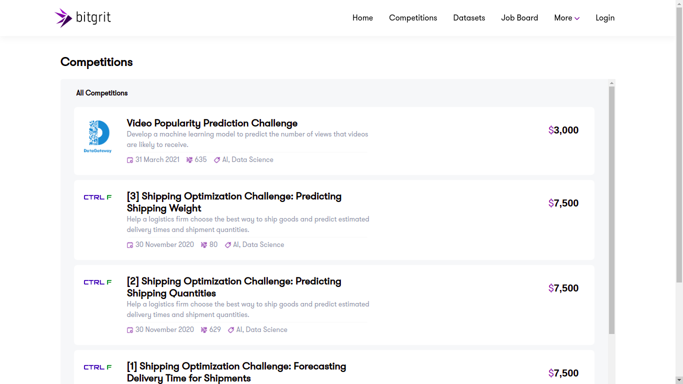
Bitgrit

Bitgrit competitions

Launched in 2019, already showing 8 competitions with various topics, this platform looks promising! As said above, it does not seem referenced on mlcontests.

bitgrit is an AI competition and recruiting platform for data scientists, home to a community of over 25,000 engineers worldwide. We are developing bitgrit to be a comprehensive online ecosystem, centered around a blockchain-powered AI Marketplace.

Drivendata

Driven data competition page

I never took part in their competitions, so I can’t say mcuh about it for now! But they have sponsored competitions.

DrivenData works on projects at the intersection of data science and social impact, in areas like international development, health, education, research and conservation, and public services. We want to give more organizations access to the capabilities of data science, and engage more data scientists with social challenges where their skills can make a difference.

Crowdanalytix

Crowdanalytix

I never took part in their competitions, so I can’t say mcuh about it for now! They seemed less active recently, but they had sponsored competitions.

25,129 + Data Scientists

102,083 + Models Built

50 + Countries

Numer.ai

https://numer.ai/

Focusing on predicting the stock market, with high quality data (which is usually a tedious task when you try to have quality data in finance). They claim to be the hardest platform in finance, and having worked there, I can confirm that finding the slightest valuable prediction is super hard!

Nice if you like finance, but be prepared to work with similar datasets!

Start with hedge fund quality data. It is clean and regularized, designed to be usable right away.

Zindi

Zindi competition page

Data science platform with competitions which are related to Africa. The NLP part seems particularly exciting, as they are focus on languages which are not studied as often as English or Spanish! Looking forward to participate in one of their challenges!

We connect organisations with our thriving African data science community to solve the world’s most pressing challenges using machine learning and AI.

Analytics Vidhya

Analytics Vidhya

India based.

Data science hackathons on DataHack enable you to compete with leading data scientists and machine learning experts in the world. This is your chance to work on real life data science problems, improve your skill set, learn from expert data science and machine learning professionals, and hack your way to the top of the hackathon leaderboard! You also stand a chance to win prizes and get a job at your dream data science company.

Challengedata

https://challengedata.ens.fr/

Not sure the competitions are sponsored here. General topics, most of them seem to come from French companies and French institutions.

We organize challenges of data sciences from data provided by public services, companies and laboratories: general documentation and FAQ. The prize ceremony is in February at the College de France.

Coda Lab

Codalab

French based.

CodaLab is an open-source platform that provides an ecosystem for conducting computational research in a more efficient, reproducible, and collaborative manner.

Topcoder

Topcoder

Not focusing only on data science:

Access our community of world class developers, great designers, data science geniuses and QA experts for the best results

InnoCentive

InnoCentive competitions

InnoCentive is the global pioneer in crowdsourced innovation. We help innovative organizations solve their important technology, science, business, A/I and data challenges by connecting them with a global network of expert problem solvers.

Datasoure.ai

Datasoure

Young company, as the quote below shows (22nd march 2021). They seem to be focused on challenges for startups, but this may evolve!

At a glance

2 Team Members

1,692 Data Scientists

12 Companies

5.2% Weekly Growth

Signate

Signate competitions

A Japanese competition platform. Most of the competitions are described in Japanese, but not all of them!

SIGNATE collaborates with companies, government agencies and research institutes in various industries to work on various projects to resolve social issues. We invite you to join SIGNATE’s project, which aims to make the world a better place through the power of open innovation.

datasciencechallenge.org (probably down)

https://www.datasciencechallenge.org/

Unfortunately, I cannot reach the website any more…

Sponsored by the Defence Science and Technology Laboratory and other UK government departments.

datascience.net (probably down for ever)

datascience.net

Used to be a French speaking data science competition for a while. However, the site has been down for a while now… Worth giving a look from time to time!

Dataviz

Here, the idea is to provide the best vizualisation of datasets. The metric may therefore not be as absolute as the one for prediction problems and the skillset is really different!

Iron viz

Iron viz

informationisbeautifulawards

informationisbeautifulawards

They are all the platforms I am aware of, if I missed any or if you have any relevant resources, please let me know!

I Hope you liked this article! If you plan to take part in any of these competitions, best of luck to you, and have fun competing and learning!