Model staging is a method that enables to produce (usually) the most competitive models, in terms of accuracy. As such, you will often find winning solutions to data science competitions to be 2-3 stages of models.

This article will assume some familiarity with cross validation. We will go through model averaging first, recall how staging works, observe the link between model averaging and model staging (also referred to as stacking or blending) and propose hypothesis (backed by some visualization) to explain why staging works so well.

Also my other post (more implementation oriented), a stacking tutorial in Python may help.

Going back to model staging, here are some verbatim about some winning solutions of data science competitions.

Per example, the Homesite quote conversion

Quick overview for now about the NMA approach:

10 variations of the dataset in total (factor combinations, factors mapped to response rates, replacing correlated pairs by differences etc) lots of models (xgboost, keras, ranger, logreg, even occasional svm - although that took forever) trained on various datasets and different params; stored as lvl1 metafeatures mix lvl1 metafeatures with: xgboost, nnet, hillclimbing, glmnet and ranger, stack - 5 lvl2 metafeatures mix the lvl2 metafeatures with hillclimbing bag at each stage as much as time permitted

Or, in the BNP Paribas Cardif Claims management:

We also produced many different base level models without much Feature engineering, just different input format types (like load all categorical variables as counts, or as onehot encoding etc).

Our ensemble was consisted of 223 models. Faron did a lot of work in removing noise and discarding many of these in order to get to our bets score with a lvl2 ensemble of geomean weights between an ET , 2NN and 2 Xgmodels.

Before understanding the mechanisms at work for model staging, let’s review the simpler “model averaging” approach.

Model averaging

What is model averaging?

Model averaging is a method that consists in averaging the predictions of different models.

It works particularly well in regression problems, or classification problem when the task consists in predicting probabilities of belonging to a specific class.

Why does averaging works?

Imagine you are facing a regression problem, and have two models. One underestimates the true value, while the other one overestimates it. In this case, the average of the two predictions will be (much) closer to the truth than each individual prediction.

The two figures below illustrate it, in the case of a squared error penalty. The x-axis represents the difference between the true value and the estimated value. The red dots are the estimations of two different models (on the x axis) and the resulting error (on the y axis). The component of the blue dot on the x-axis is the average of the components of the red dots on the x-axis.

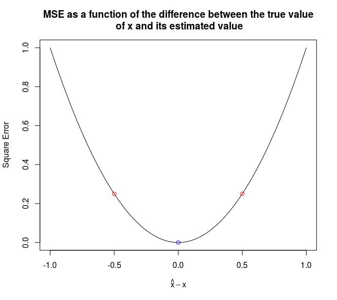
It is worth noting that blending will work better if the models have a similar performance (in terms of out-of-sample accuracy) and are as little correlated as possible.

Jensen inequality

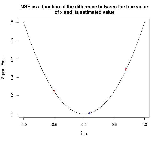
What is even better is that if both models overestimate (or underestimate) the true value, the penalty is still lower.

The graph below presents it:

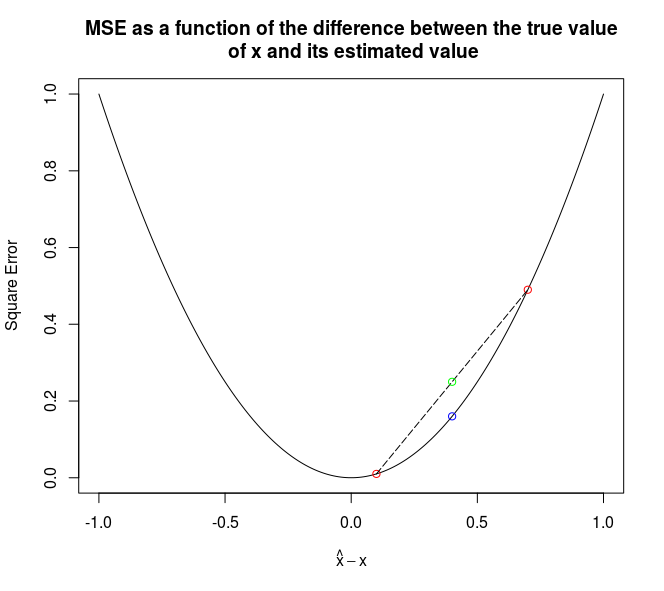
The green point correpond to the average of the errors, while the blue point correspond of the error of the average.

Proofs can be found on Wikipedia for the purpose of the article, it is enough to convice oneself that this works with these simple graphs.

Jensen’s inequality applies to convex functions, but log loss, squared error (MSE), absolute value error (MAE) are convex functions.

The R code below can be used (just change the xs_points <- c(0.1, 0.8)) to reproduce the experiment with other values.

parabola = function(x) {
  x * x
}
xs <- seq(-1, 1, 0.01)
xs_points <- c(0.1, 0.8)

plot(
  xs,
  parabola(xs),
  xlab = expression(hat(x) - x),
  ylab = "Square Error",
  type = 'l',
  main = "MSE as a function of the difference between the true value\n of x and its estimated value"
)

for (xs_point in xs_points) {
  points(x = xs_point,
         y = parabola(xs_point),
         col = "red")
}

points(x = mean(xs_points),
       y = parabola(mean(xs_points)),
       col = "blue")
segments(
  x0 = xs_points[1],
  x1 = xs_points[2],
  y0 = parabola(xs_points[1]),
  y1 = parabola(xs_points[2]), lty = 11
)
points(x = mean(xs_points),
       y = mean(parabola(xs_points)),
       col = "green")

Model stacking

Historical note

As far as I know, the first presentation of stacking goes back to 1992: Stacked generalization, by David H. Wolpert (also famous for the result no free lunch in search and optimization)

[…] The conclusion is that for almost any real-world generalization problem one should use some version of stacked generalization to minimize the generalization error rate.

And almost 30 years later, it remains true! Quoting the wikipedia page:

This work was developed further by Breiman, Smyth, Clarke and many others, and in particular the top two winners of 2009 Netflix competition made extensive use of stacked generalization (rebranded as “blending”)

How does it work?

Generalizing averaging

So far, we have seen model averaging. You take two models (or \(n\)), and average them.

On the other hand, assuming you cross validate \(n\) models and only use the best for future predictions, you have another strategy that forms one model from \(n\) models.

So we have two schemes that put weights on different models. One puts an equal weight to every model, the other one puts all the weights on the best model.

Model staging consists in using another learning algorithm to choose the “weights” to give to each model. A linear regression “on top” of other models consists in giving an “ideal” (in the regression sense) weight to each model, but what is amazing is that you may use something else than a linear regression!

Detailing staging procedure

The idea, to give a correct “weight” to each model is to perform a cross validation on the training set and return a dataset for which each element correspond to the unseen fold prediction. On this new dataset, you can fit the new model.

Per example, in the case of a regression problem, if you have \(n\) rows in your data set, \(p\) features and \(k\) models, this step turns your training data from a \(n,p\) matrix to a \(n,k\) matrix.

Thus the element with index \(i,j\) in this new matrix corresponds to the prediction of the \(i\)-th observation by the \(j\)-th model.

Why does this work?

General case of averaging

Averaging, because of Jensen’s inequality, usually improves the accuracy of the models. Staging, seen as a generalization of averaging, will also improve the accuracy of our learners.

More general decision boundaries

Hypothesis

Another argument, which could be rephrased in more scientific terms is that it allows to obtain decision boundaries of a wider shape than the ones of each usual learning algorithm.

Put another way, the supervised learning problems can be seen as finding \(f\) such that:

Where \(f\) belongs to some function space. For the linear regressions (penalized or not), \(f\) has to be a linear function, for a decision tree, \(f\) belongs to a space of sum of indicator functions, for kernel functions, \(f\) is a linear combination of kernels…

The hypothesis here is that, in the case of averaging, \(f\) can be linear in some region, constant by pieces in another, etc, making the search space for \(f\) larger than the search space of all the single families of models.

Visualization

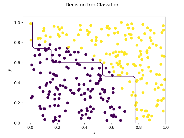
As expected, the decision tree has a decision boundary consisting of segments parallel to the x and y axis.

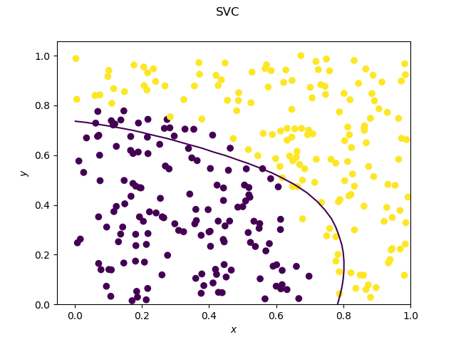
The SVC on the other hand has a very smooth decision boundary.

And here comes the magic, the decision boundary is “a little bit of both”.

Same when we blend with a decision tree.

Code

I use the default stacking proposed by scikit-learn.

First a small class useful to plot decision boundaries.

import numpy as np
import matplotlib.pyplot as plt


class DecisionBoundaryPlotter:

    def __init__(self, X, Y, xs=np.linspace(0, 1, 30),
                 ys=np.linspace(0, 1, 30)):
        self._X = X
        self._Y = Y
        self._xs = xs
        self._ys = ys

    def _predictor(self, model):
        model.fit(self._X, self._Y)
        return (lambda x: model.predict_proba(x.reshape(1,-1))[0, 0])

    def _evaluate_height(self, f):
        fun_map = np.empty((self._xs.size, self._ys.size))
        for i in range(self._xs.size):
            for j in range(self._ys.size):
                v = f(
                    np.array([self._xs[i], self._ys[j]]))
                fun_map[i, j] = v
        return fun_map

    def plot_heatmap(self, model, name):
        f = self._predictor(model)
        fun_map = self._evaluate_height(f)

        fig = plt.figure()
        s = fig.add_subplot(1, 1, 1, xlabel='$x$', ylabel='$y$')
        im = s.imshow(
            fun_map,
            extent=(self._ys[0], self._ys[-1], self._xs[0], self._xs[-1]),
            origin='lower')
        fig.colorbar(im)
        fig.savefig(name + '_Heatmap.png')
    
    def plot_contour(self, model, name):
        f = self._predictor(model)
        fun_map = self._evaluate_height(f)

        fig = plt.figure()
        s = fig.add_subplot(1, 1, 1, xlabel='$x$', ylabel='$y$')
        s.contour(self._xs, self._ys, fun_map, levels = [0.5])
        s.scatter(self._X[:,0], self._X[:,1], c = self._Y)
        fig.suptitle(name)
        fig.savefig(name + '_Contour.png')

The plots (yeah, the nested named models is not that elegant):

import numpy as np
from sklearn.ensemble import RandomForestClassifier, ExtraTreesClassifier, AdaBoostClassifier
from sklearn.tree import DecisionTreeClassifier
from sklearn.svm import SVR, SVC
from sklearn.neighbors import KNeighborsClassifier  
from sklearn.linear_model import LogisticRegression
from sklearn.ensemble import StackingClassifier
from DecisionBoundaryPlotter import DecisionBoundaryPlotter


def random_data_classification(n, p, f):
    predictors = np.random.rand(n, p)
    return predictors, np.apply_along_axis(f, 1, predictors)


def parabolic(x, y):
    return (x**2 + y**3 > 0.5) * 1


def parabolic_mat(x):
    return parabolic(x[0], x[1])


X, Y = random_data_classification(300, 2, parabolic_mat)

dbp = DecisionBoundaryPlotter(X, Y)

named_classifiers = [ (DecisionTreeClassifier(max_depth=4), "DecisionTreeClassifier"),
                     (StackingClassifier(estimators=[
                            ("svc", SVC(probability=True)), 
                            ("dt", DecisionTreeClassifier(max_depth=4))], 
                         final_estimator=LogisticRegression()), 
                         "Stacked (Linear)"),
                     (StackingClassifier(estimators=[
                            ("svc", SVC(probability=True)), 
                            ("dt", DecisionTreeClassifier(max_depth=4))], 
                         final_estimator=DecisionTreeClassifier(max_depth=4)), 
                         "Stacked (Decision Tree)"),
                     (SVC(probability=True), "SVC")]

for named_classifier in named_classifiers:
    print(named_classifier[1])
    dbp.plot_contour(named_classifier[0], named_classifier[1])

Learning more and references

The elements of statistical learning by Trevor Hastie, Robert Tibshirani, Jerome Friedman is a brilliant introduction to machine learning and will help you have a better understanding of cross validation and the learning algorithms presented here (SVC, Decision trees) but unfortunately does not treat model staging.