
The CEV Process
In mathematical finance, the CEV or constant elasticity of variance model is a stochastic volatility model which was developed by John Cox in 1975. It captures the fact that the log returns may not have a constant volatility, which the usual geometric brownian motion assumes.
The equation of the CEV model is the following.
\[dS_t = \mu S_t dt+\sigma S_t^{\gamma}dW_t\]For \(\gamma = 1\) we have the usual equation for the geometric Brownian motion:
\[dS_t = \mu S_t dt+\sigma S_t dW_t\]Simulating processes
Using the discretization method, we can simulate these processes.
Geometric Brownian motion
The geometric Brownian motion can be simulated using the following class.
import numpy as np


class ProcessGBM:

    def __init__(self, mu, sigma):
        self._mu = mu
        self._sigma = sigma

    def Simulate(self, T=1, dt=0.001, S0=1.):
        n = round(T / dt)

        mu = self._mu
        sigma = self._sigma

        gaussian_increments = np.random.normal(size=n - 1)
        res = np.zeros(n)
        res[0] = S0
        S = S0
        sqrt_dt = dt ** 0.5
        for i in range(n - 1):
            S = S + S * mu * dt + sigma * \
                S * gaussian_increments[i] * sqrt_dt
            res[i + 1] = S

        return res
Following a similar logic, we can generate trajectories for a CEV process.
import numpy as np


class ProcessCEV:

    def __init__(self, mu, sigma, gamma):
        self._mu = mu
        self._sigma = sigma
        self._gamma = gamma

    def Simulate(self, T=1, dt=0.001, S0=1.):
        n = round(T / dt)

        mu = self._mu
        sigma = self._sigma
        gamma = self._gamma

        gaussian_increments = np.random.normal(size=n - 1)
        res = np.zeros(n)
        res[0] = S0
        S = S0
        sqrt_dt = dt ** 0.5
        for i in range(n - 1):
            S = S + S * mu * dt + sigma * \
                (S ** gamma) * gaussian_increments[i] * sqrt_dt
            res[i + 1] = S

        return res
Which can then be plotted:
import matplotlib.pyplot as plt

from ProcessGBM import ProcessGBM
from ProcessCEV import ProcessCEV

T = 20
dt = 0.01
plt.plot(ProcessGBM(0.05, 0.15).Simulate(T, dt), label="GBM")
plt.plot(ProcessCEV(0.05, 0.15, 0.5).Simulate(
    T, dt), label="CEV (gamma = 0.5)")
plt.plot(ProcessCEV(0.05, 0.15, 1.5).Simulate(
    T, dt), label="CEV (gamma = 1.5)")

plt.xlabel('Time index')
plt.ylabel('Value')

plt.title("Realization of stochastic processes")

plt.legend()

plt.show()
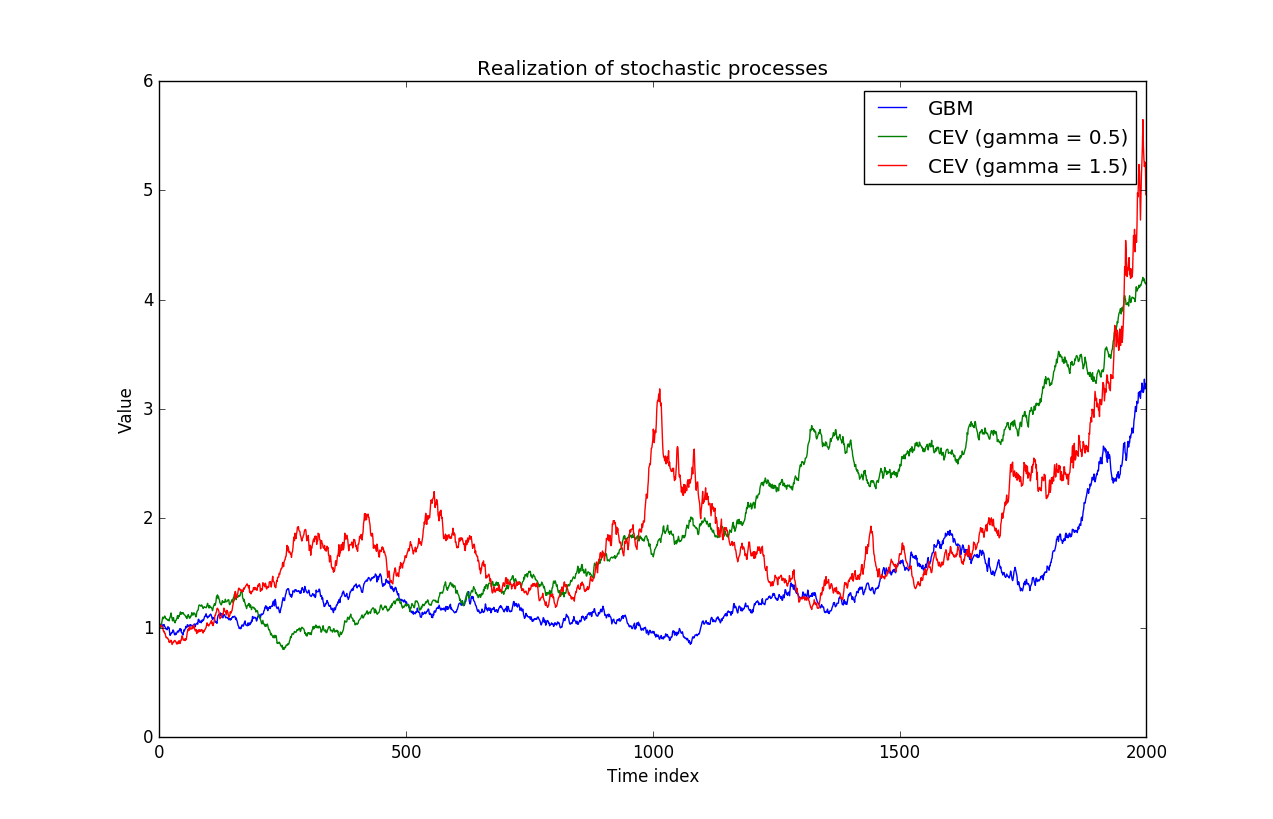
And we can “see” the properties of the trajectories, a low value for \(\gamma\) yields trajectories which are slightly linear, whereas a \(\gamma\) higher than \(1\) allows the volatility to increase for large values of the process (the trajectory in red).
Estimating the CEV parameters
Theory
A detailed method to estimate the various parameters can be found here: L. CHU, K & Yang, Hailiang & Yuen, Kam. (2001). Estimation in the Constant Elasticity of Variance Model. British Actuarial Journal. 7. 10.1017/S1357321700002233.
Note that they use slightly different notations, which will be kept in this section (the code for the estimator, however, translates everything back in terms of the original notations).
\[dS_t = \mu S_t dt+\delta S_t^{\theta / 2}dW_t\]Calling \(\sigma^2_t=\delta^2 S_t^{\theta - 2}\)
The paper recalls that \(V_t\) is an estimate of \(\sigma^2_t\), where \(V_t\) is:
\[V_t=\frac{2}{\alpha \Delta t} \left( \frac{S_{t+\Delta t}^{1+\alpha} - S_{t}^{1+\alpha}} {(1+\alpha)S_{t}^{1+\alpha}} - \frac{S_{t+\Delta t} - S_{t}} {S_{t}} \right) \frac{1}{\Delta t}\]For \(\alpha\) a constant.
It looks like there is there a typo in the original paper, after a quick implementation (see below), I realized that the estimator does not work this this formula, but does so when I remove one of the \(\frac{1}{\Delta t}\). Therefore, in what follows, the following formula will be implemented:
\[V_t=\frac{2}{\alpha \Delta t} \left( \frac{S_{t+\Delta t}^{1+\alpha} - S_{t}^{1+\alpha}} {(1+\alpha)S_{t}^{1+\alpha}} - \frac{S_{t+\Delta t} - S_{t}} {S_{t}} \right)\]Then, the variance of \(V_t\) is minimized for a value of (\(c_i\) are negative constants)
\[\alpha=c_1 + c_2\frac{\mu}{\sigma^2_t}\]And the authors suggest to start from a random value of \(\alpha\) and iterate over successive estimations of \(\mu\) and \(\sigma_t\). However, \(\sigma_t\) not being constant, this formula did not make a lot of sense to me. I chose a constant value of \(\alpha\) in the code, which provides good results.
Proof sketch : Itô’s lemma
In order to know where does \(V_t\) comes from, we can apply Itô’s formula to \(S^{1+\alpha}_t\):
\[d(S^{1+\alpha}_t)=(1+\alpha)S^{\alpha}_t dS_t + \frac{1}{2} \alpha (1+\alpha) S^{\alpha - 1}_t d<S_t>\]Now:
\[d<S_t> = \delta^2 S^{\theta}_t dt\]Therefore, dividing by \((1+\alpha)S^{1+\alpha}_t\):
\[\frac{d(S^{1+\alpha}_t)}{(1+\alpha)S^{1+\alpha}_t} - \frac{dS_t}{S_t} = \frac{1}{2} \alpha \delta^2 S^{\theta - 2}_t dt\]Finally:
\[\frac{2}{\alpha dt} \left( \frac{d(S^{1+\alpha}_t)}{(1+\alpha)S^{1+\alpha}_t} - \frac{dS_t}{S_t} \right) = \delta^2 S^{\theta - 2}_t\]And it works for any \(\alpha\). To be honest I am quite uncomfortable with the meaning to give to every equation, but, at some level, it makes sens that \(V_t\) “has to be” of the form above.
Python implementation
import numpy as np


class EstimatorCEV:

    def __init__(self, dt):
        self._dt = dt
        self._alpha0 = -5

    def Estimate(self, trajectory):
        sigma, gamma = self._evaluate_sigma_gamma(trajectory, self._alpha0)
        if sigma == None:
            return None, None, None
        else:
            mu = self._estimate_mu(trajectory)
            return (mu, sigma, gamma)

    def _log_increments(self, trajectory):
        return np.diff(trajectory) / trajectory[:-1]

    def _estimate_mu(self, trajectory):
        return np.mean(self._log_increments(trajectory)) / self._dt

    def _log_increments_alpha(self, trajectory, alpha):
        mod_increments = self._log_increments(trajectory ** (1 + alpha))
        return mod_increments / (1 + alpha)

    def _evaluate_Vt(self, trajectory, alpha):
        lhs = self._log_increments_alpha(trajectory, alpha)
        rhs = self._log_increments(trajectory)
        center = 2 * (lhs - rhs) / (alpha * self._dt)
        return center

    def _evaluate_sigma_gamma(self, trajectory, alpha):
        if np.any(trajectory <= 0):
            return None, None

        Vts = self._evaluate_Vt(trajectory, alpha)
        if np.any(Vts <= 0):
            return None, None
        logVts = np.log(Vts)

        Sts = trajectory[:-1]  # removes the last term as in eq. (5)
        if np.any(Sts <= 0):
            return None, None
        logSts = np.log(Sts)

        ones = np.ones(Sts.shape[0])
        A = np.column_stack((ones, logSts))

        res = np.linalg.lstsq(A, logVts, rcond=None)[0]
        return (2 * np.exp(res[0] / 2), 0.5 * (res[1] + 2))


if __name__ == "__main__":

    from ProcessCEV import ProcessCEV

    def test(true_mu, true_sigma, true_gamma):
        dt = 0.001
        T = 10

        sample_mu = []
        sample_sigma = []
        sample_gamma = []

        for i in range(100):
            mu_est, sigma_est, gamma_est = EstimatorCEV(dt=dt).Estimate(ProcessCEV(
                true_mu, true_sigma, true_gamma).Simulate(T, dt=dt))

            if mu_est != None:
                sample_mu = [mu_est] + sample_mu
                sample_sigma = [sigma_est] + sample_sigma
                sample_gamma = [gamma_est ] + sample_gamma

        print("mu : " + str(true_mu) + " \t| est : " + str(np.mean(sample_mu)) + " \t| std : " + str(np.std(sample_mu)))
        print("sigma : " + str(true_sigma) + " \t| est : " + str(np.mean(sample_sigma)) + " \t| std : " + str(np.std(sample_sigma)))
        print("gamma : " + str(true_gamma) + " \t| est : " + str(np.mean(sample_gamma)) + " \t| std : " + str(np.std(sample_gamma)))
        print(10*"-")


    test(0.,0.5,0.8)
    test(0.2,0.5,0.8)
    test(0.2,0.5,1.2)
    test(0.,0.3,0.2)
    test(0.,0.5,2)
Running the tests…
mu : 0.0  | est : 0.08393998598504683   | std : 0.10950360432103644
sigma : 0.5   | est : 0.5290411001633833  | std : 0.010372415832707949
gamma : 0.8   | est : 0.7995912270171245  | std : 0.023552858445145052
----------
mu : 0.2  | est : 0.21126788898622506   | std : 0.1379314635624178
sigma : 0.5   | est : 0.5295722080080916  | std : 0.01067649238716792
gamma : 0.8   | est : 0.7981059837608774  | std : 0.019084913069205692
----------
mu : 0.2  | est : 0.20468181972280103   | std : 0.16048227152782532
sigma : 0.5   | est : 0.5299253491070517  | std : 0.008389773769199063
gamma : 1.2   | est : 1.2042365895022817  | std : 0.021453412919601324
----------
mu : 0.0  | est : 0.0743428420875073  | std : 0.07189306488901058
sigma : 0.3   | est : 0.31771919915814173   | std : 0.006063917451139664
gamma : 0.2   | est : 0.2080203482037684  | std : 0.039438575768452104
----------
mu : 0.0  | est : -0.009815876356783935   | std : 0.11178850054168586
sigma : 0.5   | est : 0.5311825321732557  | std : 0.013167973885022026
gamma : 2   | est : 2.0050079526000903  | std : 0.03448408469682434
----------
It worked !
Learning more
I used to study stochastic processes a while ago and reading: Pierre Henry-Labordère – Analysis, Geometry & Modeling in Finance (which I recommend if you are interested in stochastic processes and differential geometry and mathematical finance in the same time) and [A Non-Gaussian Option Pricing Model with Skew
L. Borland, J.P. Bouchaud](https://arxiv.org/abs/cond-mat/0403022) led me to spend more time understanding them. Hence this small tuto, hope you liked it.
Financial Modelling with Jump Processes is a must read if you want to have a detailed view on the non gaussian models used for financial asset. It covers both the theoretical view of these models, the simulation and estimation procedures.