
“In Q methodology there is little more reason to understand the mathematics involved than there is to understand mechanics in order to drive a car.” S.R. Brown
Context
This methodology is particularly relevant when one wants to assess the order of importance of variables as seen by a sample of individuals. Per example “A good computer… must be fast, must be beautiful, must be resistant to shocks …”. One approach could be the usual Likert scale analysis. However, the issue is that some (many) individuals may think that every factor is very important.
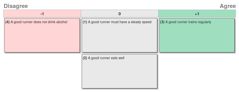
This is why, somehow, q methodology was born. It simply forces the respondant to order their preferences. How ? The assertions have to be placed in a pyramid. Then the position of each element for each participant constitutes the dataset. Each individual will fill a pyramid with different assertions, like the one below.
Who uses Q-methodology ?
Some will use q-methdology to study the conceptualization of democracy by the individuals [1] the quality of education as seen by teachers [2] or the goals and values of beef farmers in Brazil [3], to name a few published applications. But it can also be used to improve customer behavior analysis, or define relevant (at last!) opinion surveys!
A detailed example
Assertions
Imagine one is asking which assertions describe a good runner.
- A good runner must have a steady speed (speed)
- A good runner eats well (food)
- A good runner trains regularly (training)
- A good runner does not drink alcohol (alcohol)
In parenthesis are the abbreviations that will be used in the next descriptions.
Encoding the data
Once the data gathered it looks like:
| Individual | speed | food | training | alcohol |
|---|---|---|---|---|
| 1. | 0 | 0 | +1 | -1 |
| 2. | +1 | 0 | 0 | -1 |
| 3. | +1 | 0 | 0 | -1 |
| … | … | |||
| n. | 0 | +1 | 0 | -1 |
Per example the row number one would be the encoding of the responses on the first figure. Each line is called a q sort.
The method
Once the data gathered and encoded, a PCA (principal component analysis) is performed on this dataset, followed by an orthogonal rotation (usually varimax). The algebraic details can be found in [5].
In the end, the data looks like:
| Factor | 1st factor | 2nd factor | … |
|---|---|---|---|
| speed | +1 | 0 | |
| food | 0 | +1 | |
| training | 0 | -1 | |
| alcohol | -1 | 0 |
Analysis
The analysis is then performed observing the axis after the rotation. Quoting [7]
The most important aspect of the study file will nonetheless be the factor arrays themselves. These will be found in a table, ‘Item or Factor Scores’. […] The interpretative task in Q methodology involves the production of a series of summarizing accounts, each of which explicates the viewpoint being expressed by a particular factor.
Basically each factor will be a point of view (or will represent different similar points of view), shared by many individuals in the sample. This is a very first step to factor analysis and I recommend reading [7] in more details for an analysis with actual data.
Implementations
The “Q sort” data collection procedure is traditionally done using a paper template and the sample of statements or other stimuli printed on individual cards. Wikipedia.
Setting up an online survey
Unless you have a lot of time to write down the assertions on small cardboards, and take pictures of the way they are disposed on a blackboard, I recommend using an online survey ! This github repository does a nice job : easy-htmlq. You really do not need a lot of knowledge of web development to get it running :)
If you do not want to go through the hassle of using your own server, you can use a firebase service (possible with this version of the code) to keep the data and deploy the pages on Netlify or on Github pages (depending on your preferences).
Let’s have a look at the contents.
├── fonts
│   ├── glyphicons-halflings-regular.eot
│   ├── [...]
│   └── glyphicons-halflings-regular.woff
├── index.html
├── LICENSE
├── logo_center.jpg
├── logo.jpg
├── logo_right.jpg
├── README.md
├── settings
│   ├── config.xml
│   ├── firebaseInfo.js
│   ├── language.xml
│   ├── map.xml
│   └── statements.xml
├── src
│   ├── angular.min.js
│   ├── [...]
│   └── xml2json.min.js
├── stylesheets
│   ├── bootstrap.min.css
│   └── htmlq.css
└── templates
    ├── dropEventText.html
    ├── [...]
    └── thanks.html
The only things that need to be changed are in settings, which are just xml files.
statements.xml and map.xml
Corresponds to the statements to be sorted by the respondant. In the first figure, we would have used the following configuration.
<?xml version="1.0" encoding="UTF-8"?>
<statements version="1.0" htmlParse="false">
  <statement id="1">
    A good runner must have a steady speed
  </statement>
  <statement id="2">
    A good runner eats well
  </statement>
  <statement id="3">
    A good runner trains regularly
  </statement>
  <statement id="4">
    A good runner does not drink alcohol
  </statement>
</statements>
Note that map.xml must be modified accordingly:
<map version="1.0" htmlParse="false">
  <column id="-1" colour="FFD5D5">1</column>
  <column id=" 0" colour="E9E9E9">2</column>
  <column id="+1" colour="9FDFBF">1</column>
</map>
config.xml
Corresponds to other questions that can be asked (checkboxes…)
firebaseInfo.js
Where to put you firebase tokens.
// Initialize Firebase
var config = {
  apiKey: "",
  authDomain: "",
  databaseURL: "",
  projectId: "",
  storageBucket: "",
  messagingSenderId: ""
};
firebase.initializeApp(config);
var rootRef = firebase.database().ref();
language.xml
Enables you to change various elements of language.
Analysis and simulations, in R
I do not have data that I can publicly disclose, so the analysis will be on simulated data.
Let’s assume you collected the data and want to analyze it. There is an R package taking charge of the analysis [4]. Let’s have a look at it with simulated data. N will be the number of individuals, target_sort a distribution that is the “actual order of preferences” of the individuals, on which we will swap some elements accross individuals, randomly. The following code does the job.
require("qmethod")

N <- 15
target_sort <- c(-2, 2, 1, -1, 1, 0, 0, -1, 1, 0)

data <- t(replicate(N, target_sort))

for (i in 1:nrow(data))
{
  switch_indices <- sample(x = ncol(data), 2)
    tmp <- data[i, switch_indices[1]]
    data[i, switch_indices[1]] <- data[i, switch_indices[2]]
    data[i, switch_indices[2]] <- tmp
}

data <- t(data)
  rownames(data) <- paste0("assertion_", 1:10)
  colnames(data) <- paste0("individual_", 1:N)

qmethod(data, nfactors = 2)
Now let’s look at the output of qmethod. It is basically a very long console output divided in several blocks. The first block is just a summary of the parameters and the data provided to the method.
Q-method analysis.
Finished on:             Mon Apr 16 18:10:10 2018
Original data:           10 statements, 15 Q-sorts
Forced distribution:     TRUE
Number of factors:       2
Rotation:                varimax
Flagging:                automatic
Correlation coefficient: pearson
Q-method analysis.
Finished on:             Mon Apr 16 18:10:10 2018
Original data:           10 statements, 15 Q-sorts
Forced distribution:     TRUE
Number of factors:       2
Rotation:                varimax
Flagging:                automatic
Correlation coefficient: pearson
Then we have more details about the data sent to the qmethod function.
Original data :
             individual_1 individual_2 individual_3 individual_4 individual_5
assertion_1            -2            0           -2           -2           -2
assertion_2             2            2            2            0            2
assertion_3             1            1            1            1            1
assertion_4            -1           -1           -1           -1            1
assertion_5            -1            1           -1            1            1
assertion_6             0            0            0            0            0
assertion_7             0            0            0            0            0
assertion_8             1           -1            1           -1           -1
assertion_9             1            1            1            1           -1
assertion_10            0           -2            0            2            0
             individual_6 individual_7 individual_8 individual_9 individual_10
assertion_1            -2            1           -2            0            -2
assertion_2             2            2            2            2             2
assertion_3             1            1            1            1            -1
assertion_4            -1           -1           -1           -1             1
assertion_5             1            1           -1            1             1
assertion_6             0            0            0           -2             0
assertion_7            -1            0            0            0             0
assertion_8             0           -1            1           -1            -1
assertion_9             1           -2            1            1             1
assertion_10            0            0            0            0             0
The loadings. In a nutshell, they represent how close someone is to the factor column at the end of the qsort. Note that the individuals where the values -2, 2 were untouched by the random swap are the one with the highest loadings with respect to f1. This may be particularly interesting if the individual are heterogeneous, and to test wether one of them (or some of them) are actually really close to the “consensual preferences” (i.e. the principal component).
Q-sort factor loadings :
                 f1    f2
individual_1   0.93 0.085
individual_2   0.26 0.762
individual_3   0.93 0.085
individual_4   0.56 0.286
individual_5   0.43 0.553
individual_6   0.80 0.517
individual_7  -0.21 0.732
individual_8   0.93 0.085
individual_9   0.27 0.849
individual_10  0.54 0.406
 (...) See item '...$loa' for the full data.
This part is seldomly reported, I ommited some lines on purpose.
Flagged Q-sorts :
              flag_f1 flag_f2
individual_1  " TRUE" "FALSE"
[...]
individual_10 "FALSE" "FALSE"
 (...) See item '...$flagged' for the full data.
This part is seldomly reported, I ommited some lines on purpose.
Statement z-scores :
             zsc_f1 zsc_f2
assertion_1  -1.841 -0.290
[...]
assertion_10 -0.088 -0.382
At last we have the figures that will usually be reported in most papers relying on qsorts. Note that the first column corresponds (almost) to c(-2, 2, 1, -1, 1, 0, 0, -1, 1, 0) as expected! Increasing N in the code allows to recover exactly the original vector.
Statement factor scores :
             fsc_f1 fsc_f2
assertion_1      -2      0
assertion_2       2      2
assertion_3       1      1
assertion_4      -1     -1
assertion_5      -1      1
assertion_6       0     -2
assertion_7       0      0
assertion_8       1     -1
assertion_9       1      1
assertion_10      0      0
Factor characteristics:
   General factor characteristics:
   av_rel_coef nload eigenvals expl_var reliability se_fscores
f1         0.8     6       6.1       41        0.96        0.2
f2         0.8     6       5.2       35        0.96        0.2

   Correlation between factor z-scores:
       zsc_f1 zsc_f2
zsc_f1   1.00   0.52
zsc_f2   0.52   1.00

   Standard error of differences between factors:
     f1   f2
f1 0.28 0.28
f2 0.28 0.28
Distinguishing and consensus statements :
              dist.and.cons f1_f2 sig_f1_f2
assertion_1  Distinguishing -1.55      ****
assertion_2       Consensus -0.17
assertion_3       Consensus -0.08
assertion_4       Consensus  0.17
assertion_5  Distinguishing -1.50      ****
assertion_6  Distinguishing  1.07       ***
assertion_7       Consensus -0.11
assertion_8  Distinguishing  1.59      ****
assertion_9       Consensus  0.29
assertion_10      Consensus  0.29
Final words
That’s it! Q methodology is a vast topic and deserves a whole book ! Covering the theory of principal components, rotations, possibly the mathematic underlying the method, like *varimax** and the other options, detailing various surveys and how the analysis was performed, setting up tests… As I was writing this post I realized how optimistic I was when I thought I could describe the method. Anyway, I hope this will be enough for a reader to set up one’s survey and analyze it.
Sources and external sites
[1] Rune Holmgaard Andersen, Jennie L. Schulze, and Külliki Seppel, “Pinning Down Democracy: A Q-Method Study of Lived Democracy,” Polity 50, no. 1 (January 2018): 4-42.
[2] Grover, Vijay Kumar (2015, August). Developing indicators of quality school education as perceived by teachers using Q-methodology approach. Zenith International Journal of Multidisciplinary Research, 5(8), 54-65.
[3] Pereira, Mariana A., John R. Fairweather, Keith B. Woodford, & Peter L. Nuthall (2016, April). Assessing the diversity of values and goals amongst Brazilian commercial-scale progressive beef farmers using Q-methodology. Agricultural Systems, 144, 1-8.
[4] Aiora Zabala. qmethod: A Package to Explore Human Perspectives Using Q Methodology. The R Journal, 6(2):163-173, Dec 2014.
[5] H. Abdi, “Factor Rotations in Factor Analyses”
[6] A primer on Q methodology - SR Brown - Operant subjectivity, 1993 - researchgate.net
[7] S. Watts and P. Stenner, “Doing Q methodology: theory, method and interpretation,” p. 26.