Introduction
Both PCA and tSNE are well known methods to perform dimension reduction. The question of their difference is often asked and here, I will present various points of view: theoretical, computational and emprical to study their differences. As usual, one method is not “better” in every sense than the other, and we will see that their successes vastly depend on the dataset and that a method may preserve some features of the data, while the other do not.
A little bit of wording and notations
PCA stands for Principal Component Analysis
whereas tSNE stands for Stochastic Neighbor Embedding, the t itself referring to the Student-t kernel.
As “usual” we will call \(n\) the number of observations and \(p\) the number of features.
Theoretical aspects
tSNE
Quoting the authors of [1]:
Stochastic Neighbor Embedding (SNE) starts by converting the high-dimensional Euclidean distances between data points into conditional probabilities that represent similarities. The similarity of data point \(x_j\) to datapoint \(x_i\) is the conditional probability \(p_{j \vert i}\), that \(x_i\) would pick \(x_j\) as its neighbor if neighbors were picked in proportion to their probability density under a Gaussian centered at \(x_i\). For nearby datapoints, \(p_{j \vert i}\) relatively high,i whereas for widely separated datapoints, \(p_{j \vert i}\) will be almost infinitesimal.
In a nutshell, this maps your data in a lower dimensional space, where a small distance between two points means that they were close in the original space.
The method goes on defining:
As the probabilities in the original space, and \(q\) the same probability, but in the space of represented points.
Then, the divergence between these distribution is minimized using a gradient descent over the \(y\) elements:
PCA
On the other hand, PCA does not rely on a probabilistic approach to represent the points. Indeed, the approach is more geometric (or related to linear algebra): PCA looks for axis that explains as much variance as possible of the data.
Following the wikipedia article, we can have a better understanding of how it performs dimension reduction:
The transformation \(T = X W\) maps a data vector \(x_i\) from an original space of \(p\) variables to a new space of \(p\) variables which are uncorrelated over the dataset. However, not all the principal components need to be kept. Keeping only the first \(L\) principal components, produced by using only the first \(L\) eigenvectors, gives the truncated transformation
$$\mathbf{T}_L = \mathbf{X} \mathbf{W}_L$$
where the matrix \(T_L\) now has \(n\) rows but only \(L\) columns. In other words, PCA learns a linear transformation \(t = W^T x, x \in R^p, t \in R^L,\) where the columns of \(p × L\) matrix \(W\) form an orthogonal basis for the \(L\) features (the components of representation \(t\)) that are decorrelated. By construction, of all the transformed data matrices with only \(L\) columns, this score matrix maximises the variance in the original data that has been preserved, while minimising the total squared reconstruction error \(\|\mathbf{T}\mathbf{W}^T - \mathbf{T}_L\mathbf{W}^T_L\|_2^2\) or \(\|\mathbf{X} - \mathbf{X}_L\|_2^2\).
What we see here is that the total squared reconstruction error is minimized. Therefore, if two points are far away in the original space, their distance will have to be important as well once they are mapped to a lower dimensional space.
In that case, this means that after a PCA, two points are far away from each other if they were far away from each other in the original data set.
Feasability
Computational complexity
If you are not familiar with this topic, I already wrote about it in computational complexity and machine learning.
PCA can be performed quite quickly : it consists in evaluating the covariance matrix of the data, and performing an eigen value of this matrix. Covariance matrix computation is performed in \(O(p^2 n)\) operations while its eigen-value decomposition is \(O(p^3)\) operations. So, the complexity of PCA is \(O(p^2 n+p^3)\). Considering that \(p\) is fixed, this is \(O(n)\).
On the other hand, tSNE can benefit form the Barnes-Hut approximation [2], making it usable in high dimensions with a complexity of \(O(n \log n)\) (more informations can be found in the article).
Therefore, it is not obvious if a method has to be preferred to another with large datasets.
Parameters
The PCA is parameter free whereas the tSNE has many parameters, some related to the problem specification (perplexity, early_exaggeration), others related to the gradient descent part of the algorithm.
Indeed, in the theoretical part, we saw that PCA has a clear meaning once the number of axis has been set.
However, we saw that \(\sigma\) appeared in the penalty function to optimize for the tSNE. Besides, as a gradient descent is required, all the usual parameters of the gradient descent will have to be specified as well (step sizes, iterations, stopping criterions…).
Looking at the implementations, the arguments of the constructors in scikit-learn are the following:
class sklearn.decomposition.PCA(n_components=None,
                copy=True, whiten=False, svd_solver='auto',
                tol=0.0, iterated_power='auto',
                random_state=None)
The parameters mostly relate to the solvers, but the method is unique. On the other hand…
class sklearn.manifold.TSNE(n_components=2, perplexity=30.0,
                early_exaggeration=12.0, learning_rate=200.0,
                n_iter=1000, n_iter_without_progress=300,
                min_grad_norm=1e-07, metric='euclidean', init='random', verbose=0,
                random_state=None, method='barnes_hut', angle=0.5, n_jobs=None)
However, default parameters usually provide nice results. From the original paper:
The performance of SNE is fairly robust to changes in the perplexity, and typical values are between 5 and 50.
Therefore, both in terms of feasability or efforts demanded by the calibration procedure, there is no reason to prefer a method to the other.
Empirical analysis
Figures
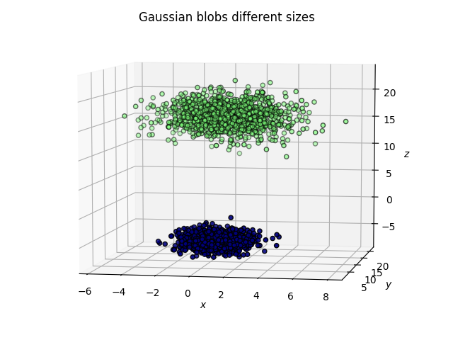
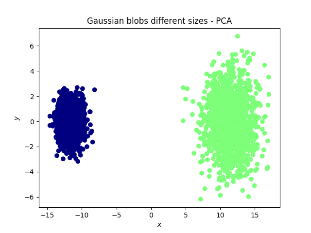
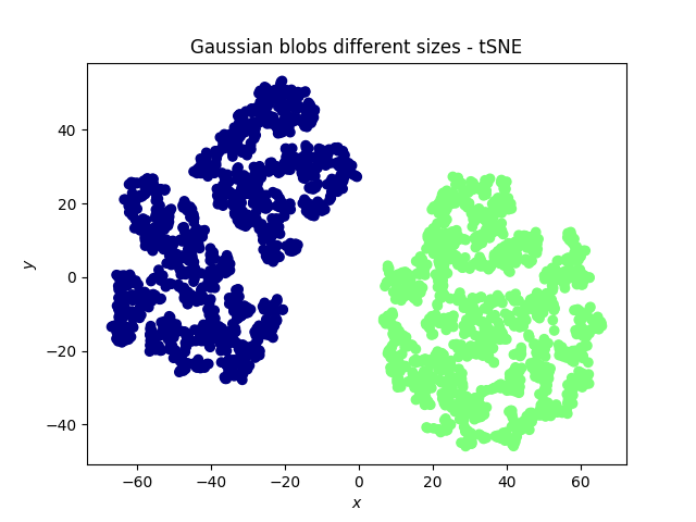
The following shows the reduction from a three dimensional space to a two dimensional space using both methods. The colors of the points are preserved, so that one can “keep track” of them.
Gaussian blobs
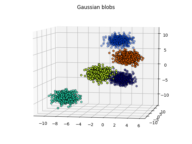
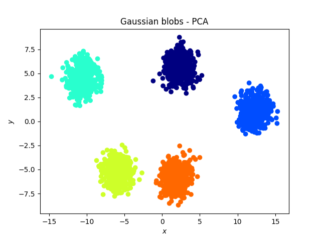
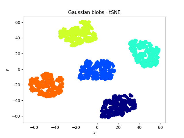
Both methods were successful at this task: the blobs, that were initally well separated, remain well separated in the lower dimensional space. An interesting phenomenon, which validates what the theoretical arguments predicted is that in the case of the PCA, the (light) blue and cyan points are far away from each other, whereas they appear to be closer when the tSNE is used.
The swiss roll
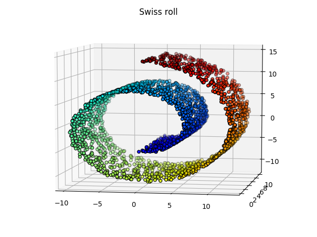
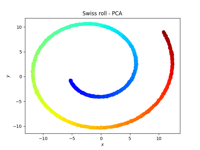
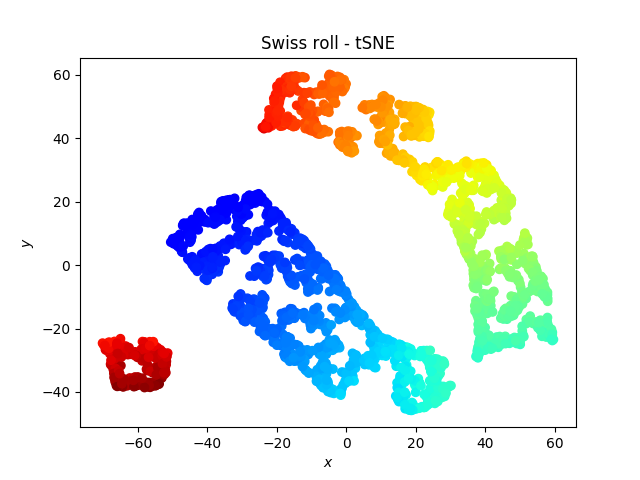
Somehow the roll is broken by the tSNE, which is weird because one would expect the red dots to be close to the orange dots… On the other hand, a linear classifier would be more successful on the data represented with the tSNE than with the PCA.
Digit dataset
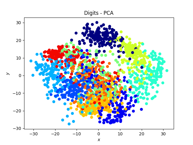
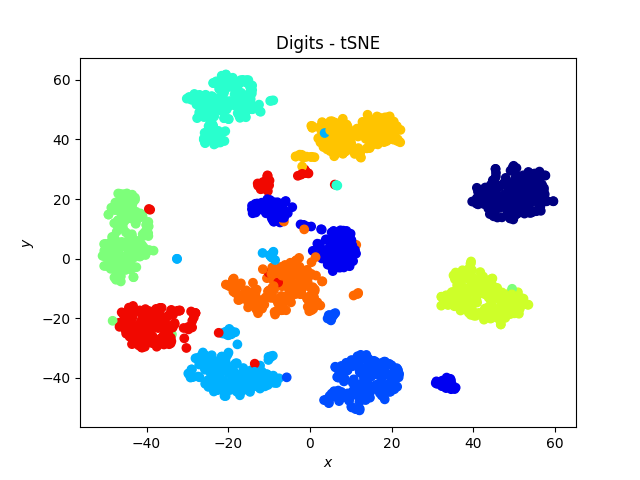
The tSNE works amazingly well on this data set, and exhibits a neat separation of most of the digits!
Hand dataset
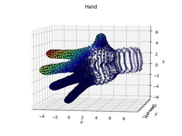
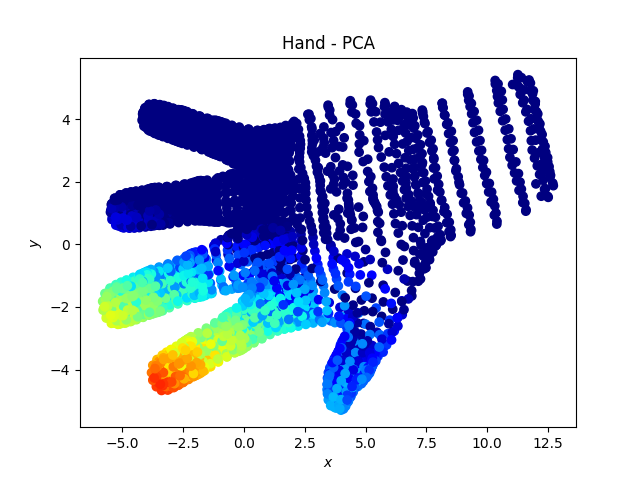
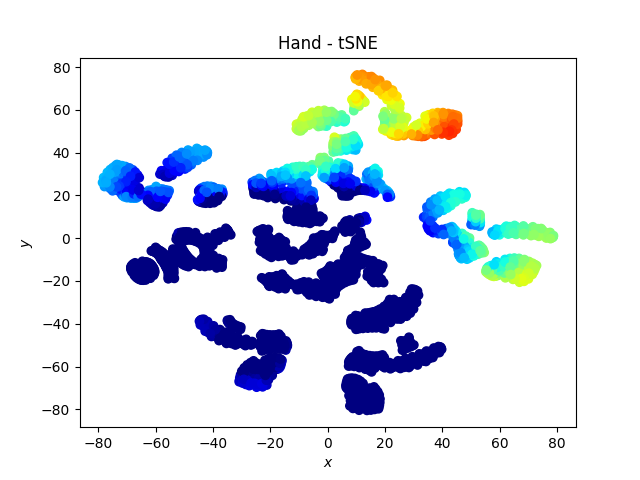
Here we note that the fingers “remain together” with the tSNE.
Other observations
Other observations could be inferred as well, per example, the size of a cluster does not mean much with the tSNE, while it has a meaning in the case of the PCA.
Code
Shall you want to explore new datasets, feel free to use the following code!
import numpy as np
import matplotlib.pyplot as plt
import mpl_toolkits.mplot3d.axes3d as p3
from sklearn.datasets import make_swiss_roll, make_blobs, load_digits
from sklearn import decomposition
from sklearn.manifold import TSNE

# Generate data (swiss roll dataset)
n_samples = 2500

def generate_swiss_roll_data(n_samples):
    noise = 0.05
    X, _ = make_swiss_roll(n_samples, noise)
    # Make it thinner
    X[:, 1] *= .5
    distance_from_y_axis = X[:, 0] ** 2 + X[:, 2] ** 2
    X_color = plt.cm.jet(distance_from_y_axis / np.max(distance_from_y_axis + 1))
    return X, X_color, "Swiss roll"

def generate_gaussian_blobs(n_samples):
    X, y = make_blobs(n_samples=n_samples, centers=5, n_features=3,random_state=3)
    X_color = plt.cm.jet(y / np.max(y + 1))
    return X, X_color, "Gaussian blobs"

def generate_gaussian_blobs_different(n_samples):
    X, y = make_blobs(n_samples=n_samples, centers=2, n_features=3,random_state=3)
    X[y == 1, :] *= 2
    X_color = plt.cm.jet(y / np.max(y + 1))
    return X, X_color, "Gaussian blobs different sizes"

def generate_digits(n_samples):
    X, y = load_digits(n_class = 10, return_X_y = True)
    X_color = plt.cm.jet(y / np.max(y + 1))
    return X, X_color, "Digits"

def generate_hand(n_samples):
    X = np.loadtxt("./Hand.csv", delimiter=",")
    z_component =  X[:, 2] - X[:, 0]
    X_color = plt.cm.jet(z_component / np.max(z_component + 1))
    return X, X_color, "Hand"


def produce_plots(data_generator, data_generator_name):
    X, X_color, title = data_generator(n_samples)
    fig = plt.figure()
    ax = p3.Axes3D(fig)
    ax.view_init(7, -80)
    ax.scatter(X[:, 0], X[:, 1], X[:, 2],
            color = X_color,
            s=20, edgecolor='k')
    ax.set_xlabel('$x$')
    ax.set_ylabel('$y$')
    ax.set_zlabel('$z$')
    plt.title(title)
    plt.savefig(data_generator_name + '.png')

    # Fit and plot PCA
    X_pca = decomposition.PCA(n_components=2).fit_transform(X)
    fig = plt.figure()
    s = fig.add_subplot(1, 1, 1, xlabel='$x$', ylabel='$y$')
    s.scatter(X_pca[:, 0], X_pca[:, 1], c = X_color)
    plt.title(title + " - PCA")
    fig.savefig(data_generator_name  + '_pca.png')

    # Fit and plot tSNE
    X_tsne = TSNE(n_components=2).fit_transform(X)
    fig = plt.figure()
    s = fig.add_subplot(1, 1, 1, xlabel='$x$', ylabel='$y$')
    s.scatter(X_tsne[:, 0], X_tsne[:, 1], c = X_color)
    plt.title(title + " - tSNE")
    fig.savefig(data_generator_name + '_tsne.png')

produce_plots(generate_digits, "digits")
produce_plots(generate_hand, "hand")
produce_plots(generate_swiss_roll_data, "swiss_roll")
produce_plots(generate_gaussian_blobs, "blobs")
produce_plots(generate_gaussian_blobs_different, "blobs_diff")
Learning more
References
[1] van der Maaten, L.J.P.; Hinton, G.E. Visualizing High-Dimensional Data Using t-SNE. Journal of Machine Learning Research 9:2579-2605, 2008.[
[2] L.J.P. van der Maaten. Accelerating t-SNE using Tree-Based Algorithms. Journal of Machine Learning Research 15(Oct):3221-3245, 2014. https://lvdmaaten.github.io/publications/papers/JMLR_2014.pdf
Related books
The elements of statistical learning by Trevor Hastie, Robert Tibshirani, Jerome Friedman is a brilliant introduction to the topic and will help you have a better understanding of most of the PCA.
Python data science handbook
Websites
Distill article on tSNE