– layout: post title: “R Kernlab (caret) VS e1071” date: 2018-06-10 14:05:43 +0100 categories: statistics tags: R svm image: feature: kernlab-vs-e1071.jpg comments: true —

A little bit of context

After seeing plenty of “Python VS Java for data science”, questions that seemed ways to broad, I decided to focus on various benchmarks for different tasks. Today will be about Support Vector Machines, in R.

There are two main packages for SVMs in R : kernlab and e1071.

While kernlab implements kernel-based machine learning methods for classification, regression, clustering, e1071 seems to tackle various problems like support vector machines, shortest path computation, bagged clustering, naive Bayes classifier.

Difference between the SVM implementations

Proposed kernels

As kernlab focuses on kernel methods, many of them are implemented:

• rbfdot Radial Basis kernel function “Gaussian”
• polydot Polynomial kernel function
• vanilladot Linear kernel function
• tanhdot Hyperbolic tangent kernel function
• laplacedot Laplacian kernel function
• besseldot Bessel kernel function
• anovadot ANOVA RBF kernel function
• splinedot Spline kernel
• stringdot String kernel

While e1071 proposes the following:

• linear
• radial basis
• polynomial
• sigmoid

Solver

e1071 relies on libsvm, which last update was released on December 22, 2016.

On the other hand, ksvm uses John Platt’s SMO algorithm for solving the SVM QP problem an most SVM formulations.

These may have an impact on the training time of these models (hopefully, the solutions should be the same).

Testing it

Unfortunately, the names of the parameters are quite different between the two libaries are not exactly the same.

This has been an issue for some users.

The radial basis kernel in e1071 is defined as \(k(u,v) = \exp(-\gamma \Vert u-v \Vert ^2)\) and as \(k(x,x") = \exp(-\sigma \Vert x-x" \Vert ^2)\). This is good. However, note that the \(C\) (cost) parameters are called C and cost.

Besides, there are many models which are available (epsilon regressions, nu regressions…) and the default behavior is not always obvious.

At last, there have been many heuristics developed to chose the best “bandwith” (referred to as \(\gamma\) and \(\sigma\) depending on the package), and the proposed heuristics are not always the same. The code below makes sure the methods match when enough parameters are provided.

require("kernlab")
require("e1071")

N <- 1000
P <- 20
noise <- 3

X <- as.matrix(matrix(rnorm(N * P), nrow = N))
Y <- as.vector(X[, 1] + X[, 2] * X[, 2] + noise * rnorm(P))

model_kernlab <-
  kernlab::ksvm(
      x = X,
      y = Y,
      scaled = TRUE,
      C = 5,
      kernel = "rbfdot",
      kpar = list(sigma = 1),
      type = "eps-svr",
      epsilon = 0.1
      )

model_e1071 <- e1071::svm(x = X,
      y = Y,
      cost = 5,
      scale = TRUE, 
      kernel = "radial",
      gamma = 1,
      type = "eps-regression",
      epsilon = 0.1)

Let”s make sure the model match.

> mean(abs(
+   predict(object = model_e1071, newdata = X) - predict(object = model_kernlab, newdata = X)
+ ))
[1] 1.254188e-14
> 
> sum(abs(predict(object = model_e1071, newdata = X) - Y))
[1] 380.0338
> sum(abs(predict(object = model_kernlab, newdata = X) - Y))
[1] 380.0338

Benchmarking

Results

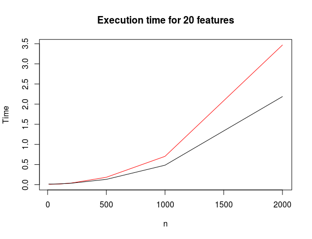
Now that we know the algorithms propose the same results, we can (safely) compare the time of execution.

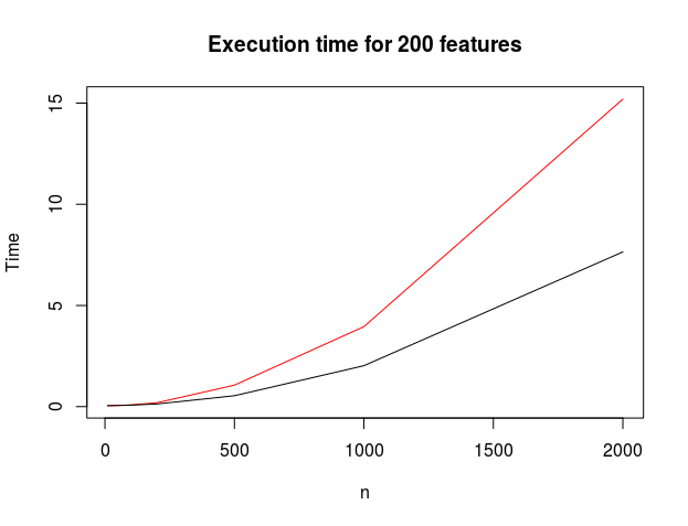
Given the success of libsvm, I expected e1071 to be faster than kernlab. The heuristics implementend to optimize the quadratic form with its constraints are not the same, (see [1] and [2]) and they may actually lead to different results on other data sets.

Learning more

[1] C.-C. Chang and C.-J. Lin, “LIBSVM: A library for support vector machines,” ACM Transactions on Intelligent Systems and Technology, vol. 2, no. 3, pp. 1–27, Apr. 2011.

[2] J. C. Platt, “Sequential Minimal Optimization: A Fast Algorithm for Training Support Vector Machines,” p. 21.

Applied predictive modelling is also good introduction to predictive modelling, with R.

The elements of statistical learning by Trevor Hastie, Robert Tibshirani, Jerome Friedman

Code

If you want to reproduce the results, the whole code is below:

require("kernlab")
require("e1071")

fit_e1071 <- function(X, Y) {
  e1071::svm(
    x = X,
    y = Y,
    cost = 5,
    scale = TRUE,
    kernel = "radial",
    gamma = 1,
    type = "eps-regression",
    epsilon = 0.1
  )
}

fit_kernlab <- function(X, Y) {
  kernlab::ksvm(
    x = X,
    y = Y,
    scaled = TRUE,
    C = 5,
    kernel = "rbfdot",
    kpar = list(sigma = 1),
    type = "eps-svr",
    epsilon = 0.1
  )
}

time_e1071 <- c()
time_kernlab <- c()

steps <- c(10, 20, 50, 100, 200, 500, 1000, 2000)

for (n in steps)
{
  noise <- 3
  P <- 20
  
  X <- as.matrix(matrix(rnorm(n * P), nrow = n))
  Y <- as.vector(X[, 1] + X[, 2] * X[, 2] + noise * rnorm(n))
  
  time_e1071 <- c(time_e1071, system.time(fit_e1071(X, Y))[1])
  time_kernlab <- c(time_kernlab, system.time(fit_kernlab(X, Y))[1])
}

plot(
  steps,
  time_e1071,
  type = "l",
  col = "red",
  xlab = "n",
  ylab = "Time",
  main = paste0("Execution time for ", P, " features"))
lines(steps, time_kernlab)